When Is the Government Spending Multiplier Large?

Lawrence Christiano, Martin Eichenbaum and Sergio Rebelo, “When Is the Government Spending Multiplier Large?” — written from the published version in the Journal of Political Economy, vol. 119 no. 1 (February 2011), pp. 78–121. No talk video for this paper exists on YouTube, so there is no transcript, discussant, or Q&A behind what follows; everything here comes from the paper.

A number about the central bank

Here is how a government spending multiplier is supposed to work, and why economists spent thirty years concluding it was boring.

You are a government. You buy a billion dollars of things — roads, aircraft carriers, the labor to build them. Mechanically, GDP goes up by a billion, because government purchases are one of the things GDP counts. The question is whether it goes up by more than a billion, and the answer depends entirely on what everyone else does in response. Your billion has to be paid for eventually, so households, being forward-looking and rather grim about it, feel poorer and spend less. Meanwhile all that new demand pushes up output, which pushes up marginal cost, which pushes up inflation, and the central bank — which has a Taylor rule and opinions — raises the interest rate. Higher real rates mean less private consumption and less private investment. Your billion elbows other spending out of the way. The multiplier lands somewhere south of one, and the fiscal-policy chapter of the textbook ends on a shrug.

There is a nice way to say this. Write the multiplier in terms of what happens to consumption, which is equation 19 in the paper:

where $g$ is the government’s share of output and hats are percentage deviations. The multiplier exceeds one if and only if private consumption goes up when the government spends. In a frictionless model it doesn’t, so it doesn’t. In a standard sticky-price model it can, barely; with Christiano, Eichenbaum and Rebelo’s benchmark calibration the multiplier under a Taylor rule is 1.05, and they report that it is hard to push above 1.2 without abusing the parameters.

Notice what did the crowding out in that story. It wasn’t scarcity, and it wasn’t the government’s balance sheet. It was the central bank. The multiplier is not really a fact about government spending. It is a fact about the monetary policy rule, wearing government spending as a disguise.

The bad state

So now break the central bank.

The shock in the paper is an increase in everyone’s discount factor — a sudden collective urge to save, which is what a financial crisis feels like from inside a household. In the simple model there is no capital, so aggregate saving must equal zero in equilibrium. Something has to make people stop wanting to save. Normally the real interest rate falls until they do.

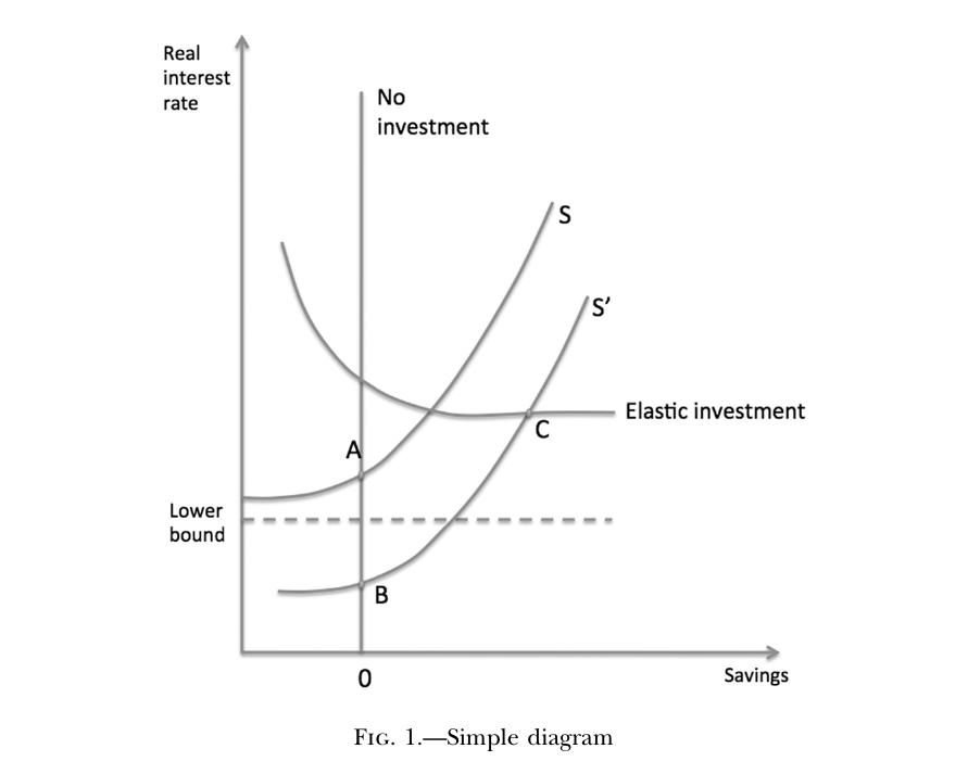
Except the real rate is the nominal rate minus expected inflation, the nominal rate stops at zero, and here the mechanism turns on itself. Output falls, marginal cost falls, prices fall. With staggered price setting, today’s price cuts are tomorrow’s expected price cuts, so agents expect deflation. Expected deflation with a nominal rate pinned at zero means the real interest rate goes up. Which makes people want to save more. Which requires output to fall further to choke off the saving. Which produces more deflation.

This is the paradox of thrift with a deflationary spiral bolted on, and the paper’s contribution is not that it exists — Krugman, Eggertsson and Woodford got there first — but what it implies about the government.

Fiscal policy as monetary policy in a borrowed coat

Run the spending increase again in this state. Government purchases rise, output rises, marginal cost rises, expected inflation rises. The nominal rate is stuck at zero, so the real rate falls — one for one with expected inflation, because nothing is absorbing it. Lower real rates raise private spending. That raises output and marginal cost again, and expected inflation again, and the real rate falls again. The same loop that was eating the economy now runs in reverse and works for you.

At the benchmark calibration, the multiplier goes from 1.05 to 3.7.

The thing to see is that the spending is almost incidental to this. What the government is producing is not roads; it is expected inflation, which is the only free variable left once the nominal rate is at zero. Fiscal policy is doing monetary policy through the Phillips curve because monetary policy can’t reach the pedal. Every subsequent result in the paper falls out of that one observation.

The multiplier is the recession, read twice

The paper’s closed form makes the point better than prose does. Let $\Theta$ be the drop in output caused by the discount-rate shock when the government does nothing. Then the zero-bound multiplier is (equation 33):

Here $p$ is the probability of staying in the trap, $\kappa$ the slope of the Phillips curve, $\beta$ the discount factor, $r^l$ the shocked discount rate, $\gamma$ and $\sigma$ preference parameters, and $g$ the government share of output. The multiplier is proportional to the disaster. Not correlated with it, not associated with it in simulations — proportional to it, in the same expression, driven by the same denominator $\Delta$ that shows up in both. Parameter values that make the zero-bound state catastrophic are exactly the parameter values that make government spending powerful, because they are the same parameter values doing the same job in both directions.

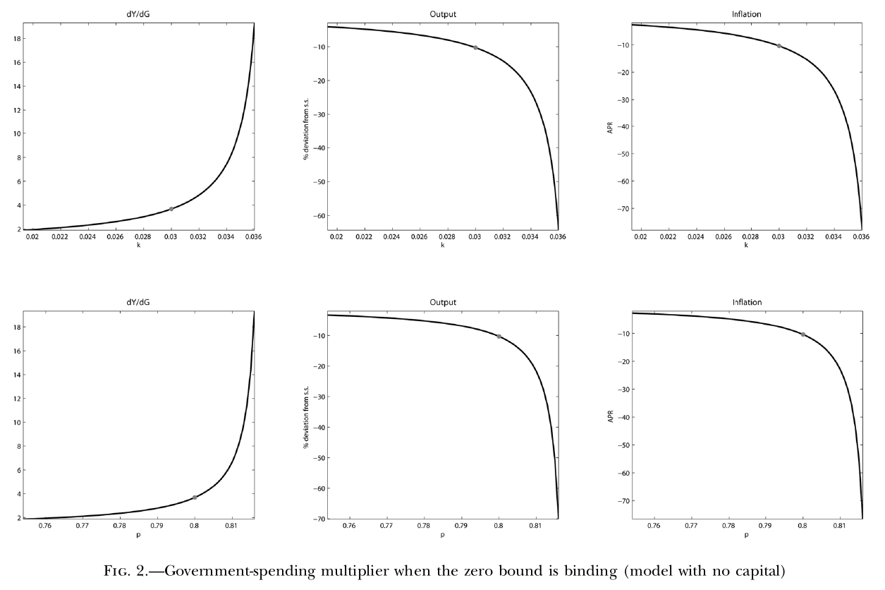
Which is a genuinely useful result and also, if you look at the left column of that figure honestly, a warning. The multiplier reaches 18 in the same place where output falls sixty percent. That is not a recession, that is the model’s denominator going to zero, and the paper says so: the necessary condition for the zero bound to bind at all is $\Delta > 0$, and everything interesting happens as $\Delta$ approaches it from above. The benchmark point is already an economy losing ten percent of output. The honest reading is not “the multiplier is 3.7” but “the multiplier and the catastrophe are the same number, so if you believe one you have to believe the other.”

Which state of the world the concrete gets poured in

The standard objection to fiscal stimulus is that it arrives late — the shovel-ready project turns out to be shovel-adjacent, and by the time the money moves the recession is over. The paper takes this seriously and gets an answer sharper than the objection.

Delay the spending by one period, and today’s output still responds, because a promise of future spending in the trap is a promise of future inflation, which lowers today’s real rate. Formally (equation 36):

The multiplier is literally the derivative of expected inflation with respect to future spending, scaled up. Its value at the benchmark is 1.5. Two periods of delay gives 1.44 — the decay is slow. But money that arrives only after the economy escapes the zero bound has a multiplier of 0.46, worse than doing nothing clever at all.

So the constraint is not speed, it is the state of the world at delivery. Late spending isn’t diluted; it’s a different policy. And a stimulus that dribbles on past the exit doesn’t merely waste the tail — in the medium-scale model it drags the whole path down.

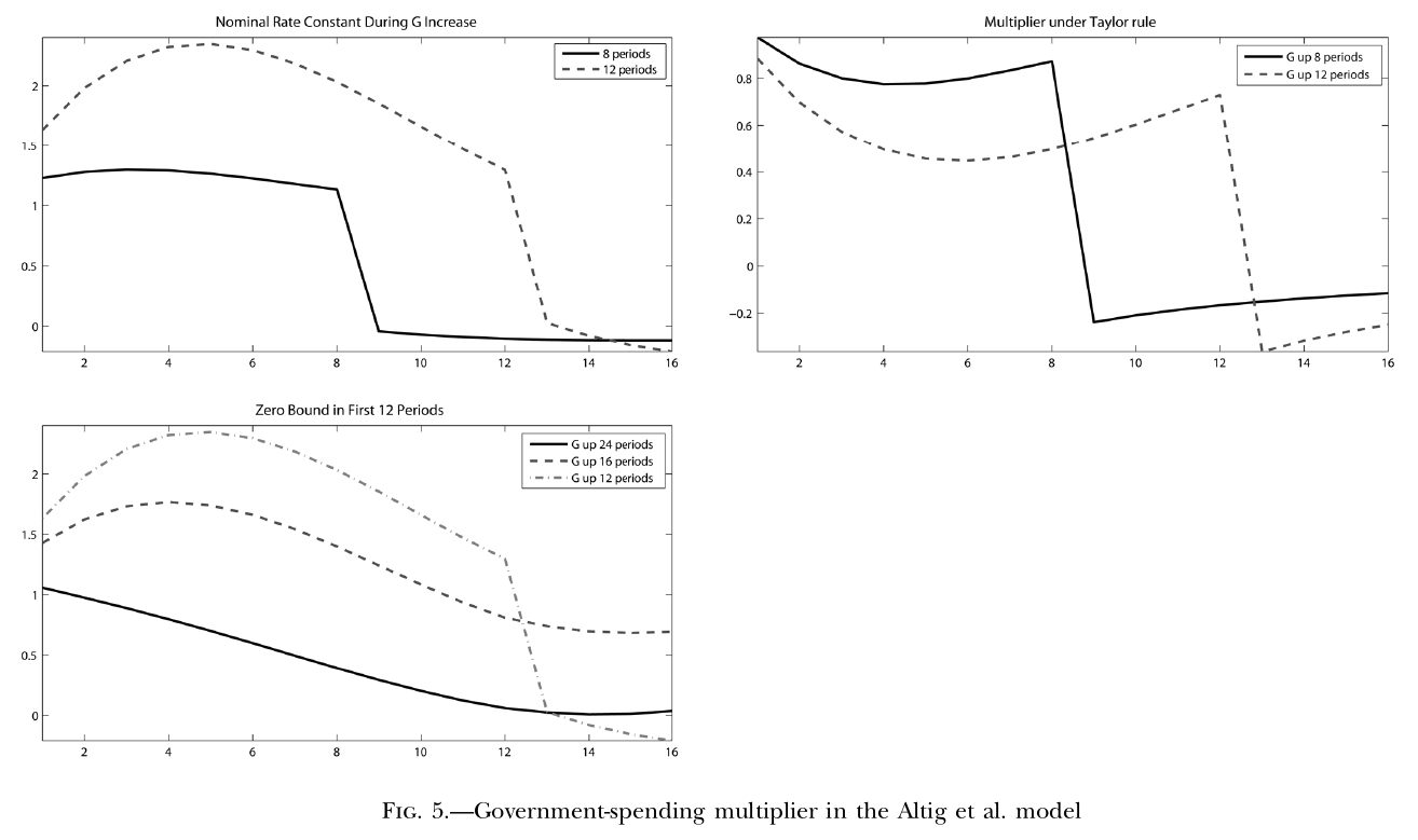
That last panel is the practical result. Take the estimated Altig–Christiano–Eichenbaum–Lindé model — sticky wages, sticky prices, habits, variable utilization, investment adjustment costs, a Phillips-curve slope of 0.0026, which is very flat — and hold the nominal rate at zero for twelve quarters. Spend over twelve quarters, all of it inside the trap: impact multiplier 1.6, peak 2.3. Spend the same amount over twenty-four quarters, half of it inside: peak 1.06. Same spending, same first twelve quarters, less than half the effect, because the part that lands outside the trap is competing with a central bank that has woken up.

(The published paper’s introduction summarizes this third finding backwards — it says the larger the fraction of spending inside the constant-rate window, the smaller the multiplier, which contradicts both its own abstract and Section V. It is a typo, and figure 5 settles it.)

Then they point it at 2008

The last section fits the model to the crisis. They date the break at 2008Q3, hit the model with the discount-factor shock plus a financial-friction shock calibrated to a 3.6-percentage-point jump in the three-year corporate spread, and compare against a univariate forecast made with data through 2008Q2.

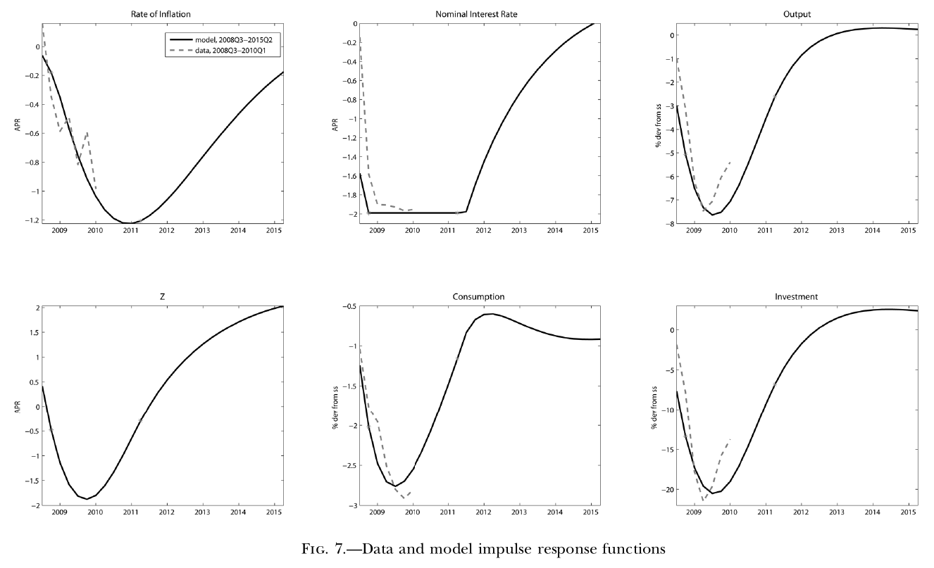
It fits well, including the part that usually doesn’t: inflation. A great many models of 2008 either produce no deflation or produce far too much; this one lands on roughly one percentage point, which is what happened. The zero bound binds in the model from 2008Q4 through 2011Q3, which is also roughly what happened.

And then the punchline, which the authors deliver in three sentences and then leave alone. In the model, as in the data, total government consumption rose by about two percent. Two percent. Despite the American Recovery and Reinvestment Act, because much of ARRA was transfers rather than purchases, and because state and local governments were cutting at the same time the federal government was spending. Multiply a two percent increase in $G$ by a peak multiplier of 2.3 at a government share of fifteen percent, and you get at most a 0.7 percent rise in annual GDP. The paper’s own summary: “The modest contribution of government purchases to the recovery reflects the very modest increase in government spending rather than a small multiplier.”

One more thing they refuse to do

The obvious next move, once you have a model saying the multiplier is 3.7 in the trap and 1.0 outside it, is to go estimate it. The paper declines, and explains why with unusual bluntness. You cannot pool the two states, because the parameter you want differs across them. And within the trap, you cannot identify exogenous movements in government spending, because spending is precisely what governments increase when output collapses. They put the problem in a footnote: suppose a government spends exactly enough to hold output constant. An econometrician regressing output on spending would find a multiplier of zero. Japan spent a great deal in the 1990s and did not grow quickly, and that observation, they note, tells you nothing whatsoever about the counterfactual.

So the paper is asking you to accept a structural model’s answer to a question that cannot be answered by the reduced-form methods you would normally trust more. It is upfront about this, which is the right thing to do and also does not make the trade any less uncomfortable.

Which leaves the reader in a position the paper doesn’t quite state. The multiplier is large exactly when the recession is severe, the recession is severe exactly when the model’s denominator is close to blowing up, and you cannot check any of this against data because the data can’t identify it. Everything hangs together. Everything hangs together because it’s the same handful of parameters appearing in every expression, which is what “internally consistent” means and also what “unfalsifiable” means, depending on your mood. The reassuring part is the smallest number in the paper: whatever the multiplier was in 2009, government purchases went up two percent, and so the question was mostly academic in the least flattering sense of the word.