Foreign Exchange Risk Management Spillovers Across the Production Network

Wentong Chen (Santa Clara University), “Foreign Exchange Risk Management Spillovers Across the Production Network,” nber conference draft dated October 9, 2026. An earlier version was Chen’s job-market paper, then titled “Foreign Exchange Risk Management Across the Production Network” and coauthored with Jisu Hwang. It was presented at imim Rising Stars in January 2025, with audience questions but no formal discussant. The October 2026 draft was presented at the nber International Finance and Macroeconomics Program Meeting on October 23, 2026, with Adrien Verdelhan as discussant; the last section covers that session. This digest follows the October 2026 draft.

Wentong Chen’s paper is about why a U.S. firm that never touches a foreign currency should care whether its suppliers buy currency forwards, and the answer turns out to be that a currency hedge is really a hedge on your borrowing rate, and your borrowing rate is part of somebody else’s input price.

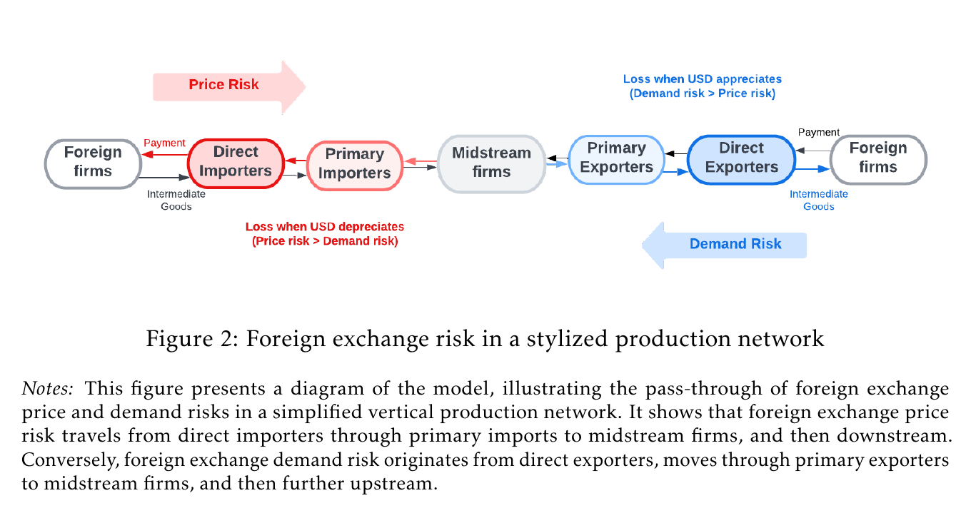
Start with the standard reassurance. U.S. trade is almost entirely invoiced in dollars: 93% of imports and 97% of exports, the paper says (p. 1). So American firms supposedly carry little currency risk. But dollar invoicing removes transaction exposure, not economic exposure. If you export a dollar-priced machine and the dollar appreciates, your foreign customer now pays more in her own currency and buys fewer machines. That is demand risk, and the invoice currency has nothing to say about it. If you import an input priced in dollars, the dollar price still drifts with the exchange rate. That is price risk. And if you are a midstream firm with no foreign customers or suppliers at all, you inherit both anyway: price risk comes down the chain from the importers, demand risk comes up it from the exporters.

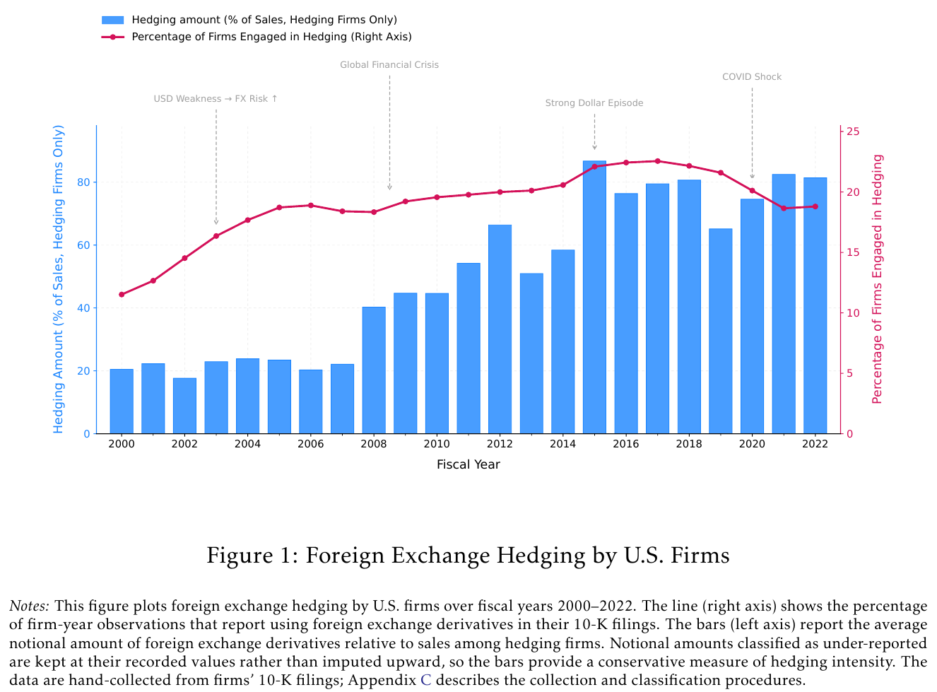
Firms act as though they know this. Chen hand-collected foreign exchange derivative notionals from 10-K filings for U.S. nonfinancial firms over fiscal 2000–2022, and the share of firms using them rises from about 12% to a peak near 22% around 2017, ending near 19%. Among hedgers, the average notional goes from about 20% of sales to somewhere between 65% and 87% after 2015. (The text says “about 60 percent,” which is more modest than the bars in its own Figure 1; trust the chart.) So a lot of firms are hedging a risk that the invoicing statistics say they don’t have.

The model: a hedge is a trade in your own credit spread

You need a reason for a firm to hedge at all, since Modigliani–Miller (1958) says it shouldn’t bother. Chen’s reason is deliberately mild. A firm borrows its entire variable production bill, inputs plus labor, before it collects any revenue (eq 5). The lender quotes a rate after the currency state is known, and that rate falls smoothly and convexly with the firm’s projected operating net worth before interest, $z = v + py - b$: resources on hand, plus expected revenue, minus the bill. There is no borrowing limit, no default, no rationing. Credit is always available; it just gets more expensive as you look weaker:

This is eq 8 in the paper: $r$ is the gross rate firm $k$ in industry $i$ pays in state $s$, $\tau$ marks whether its price is preset (rigid) or flexible, $R_{\min}$ is the floor, $\Delta R$ the premium at a reference position $z^0$, $\mathrm{Rev}^0_i$ a revenue scale, and $\gamma$ the steepness, the one parameter the calibration chooses to fit the data.

The consequence is that a dollar is worth more than a dollar. An extra dollar of resources in some state raises $z$, which lowers the rate on the whole financed bill. So you would like to move dollars from states where your rate is low anyway to states where it is high, and a fairly priced currency forward (expected payoff zero, with a small convex cost) is precisely a tool for moving dollars across exchange-rate states. The optimal position is the covariance of the marginal value of resources with the exchange rate:

These are eqs 23 and 25 in the paper: $m$ is the value of one more dollar in state $s$, $b$ the financed bill, $\psi = -R'(z)$ the slope of the credit schedule, $\zeta$ how much a dollar raises $z$ (one for a rigid-price firm), $q^*$ the signed forward position (long pays when the dollar depreciates), $c$ the hedge-cost coefficient and $e(s)$ dollars per unit of foreign currency.

Two things fall out. First, with a flat credit schedule $m \equiv 1$ and nobody hedges, which is the Modigliani–Miller benchmark recovered as a special case. Second, the hedge direction is set by where dollars are valuable, not by the sign of your exposure. In the paper’s two-state rigid-price example (App A.4.2, a set of sufficient conditions rather than a general theorem), the importer goes long, as you’d expect. The exporter goes short only if the credit schedule is steep enough, condition (A9). If the inequality runs the other way, the exporter goes long, because its financed bill is biggest in the high-demand state, so that is where a dollar saves the most interest; and the privately optimal hedge then raises the dispersion of its net worth. So a firm can hedge rationally and become less stable. The paper is careful that this is local, that Prop 3 presumes an interior optimum, and that the rigid-type ordering alone does not pin down a firm that may end up either type. But it is a nice reminder that “hedging” is a word for a trade, not a word for an outcome.

Now the network. The rate is part of marginal cost: a flexible-price firm sets $p_F = M\,r\,C$ (eq 17), markup times borrowing rate times unit cost. So a supplier sector that hedges has a steadier rate across states, hence a steadier price, hence its customers face a steadier input cost (downstream, Prop 5). A customer sector that hedges has a steadier rate, steadier output, hence steadier orders to its suppliers (upstream, Prop 6). Firms are atomistic, so, in the paper’s words, “a single counterparty’s hedge does not move sector prices or quantities” (p. 19); it is the supplier or customer sector as a whole that matters, and no individual firm counts these effects when it picks its hedge. It is a pecuniary externality. Chen is explicit that this does not, by itself, establish strategic complementarity or a welfare inefficiency (p. 8), and that the stabilizing sign of Props 5 and 6 is conditional (other terms held fixed; a short hedge by the exporting customer).

The evidence: your counterparties start hedging, your numbers calm down

The empirical design is a matched event study. The treatment is the first year in which a firm goes from having no observed hedging supplier (or customer) to having at least one, using Compustat Segment major customers and FactSet Revere links over 2003–2022. Each treated firm is matched one-to-one, with replacement, to a firm in the same treatment year and industry whose network shows no hedging from $T-1$ through $T+3$, matched on size, leverage, cash, tangibility, trade credit, own hedging, and pre-period outcome levels and slopes. The outcome is “volatility” in a specific and slightly generous sense: the absolute annual log change in sales or cost of goods sold. It is a one-year growth rate in absolute value, not a rolling standard deviation and not an exchange-rate residual, so it picks up all kinds of volatility, currency-driven or not.

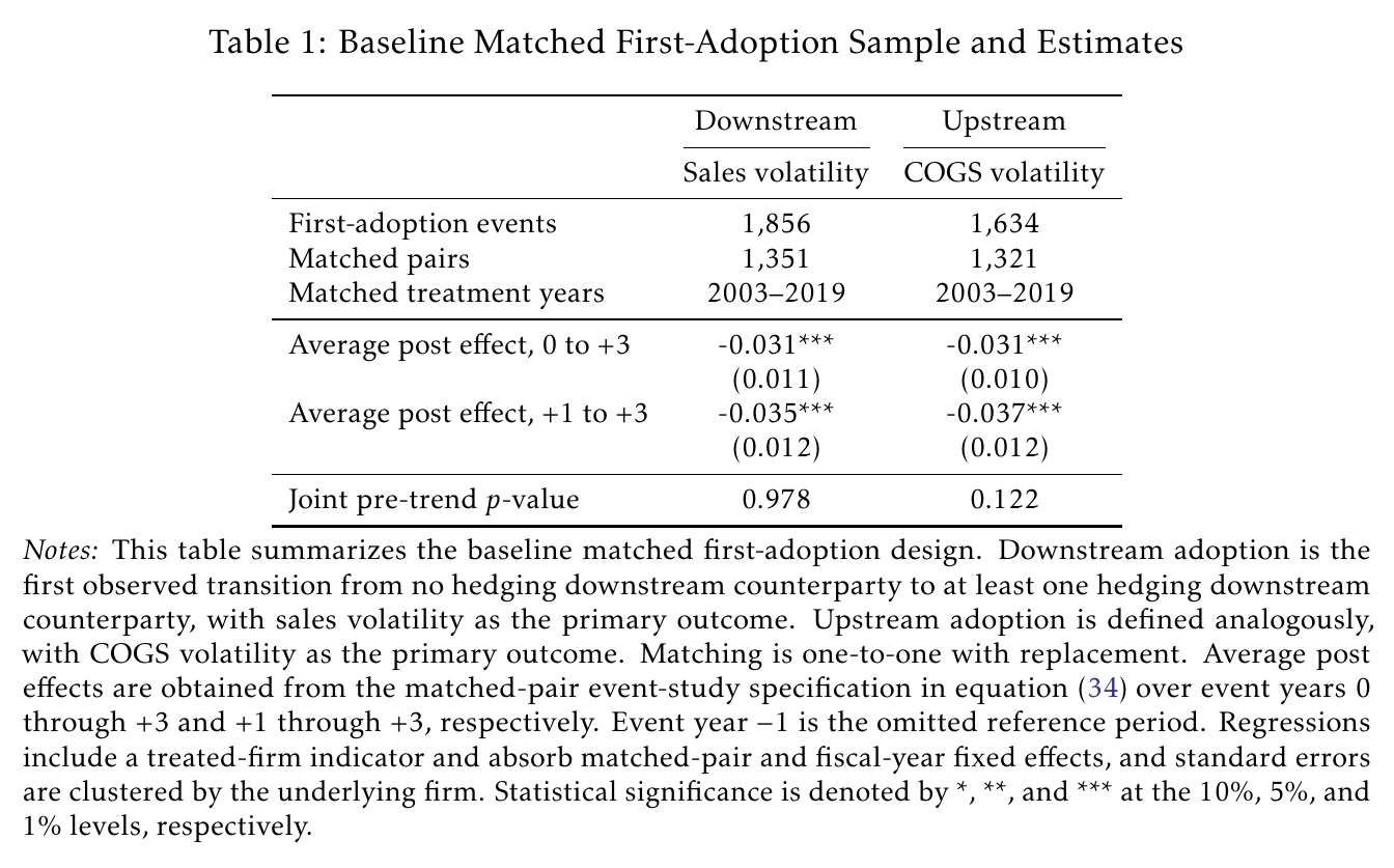
With 1,351 matched pairs on the customer side and 1,321 on the supplier side, the average post-event effect over years 0 to +3 is −0.031 for both: when customers start hedging, a firm’s absolute sales growth falls by 3.1 percentage points (standard error 0.011); when suppliers start hedging, its absolute cogs growth falls by the same 3.1 points (standard error 0.010). Against treated firms’ pre-event levels, that is 12–14%. The joint pre-trend test does not reject (p = 0.978 downstream, 0.122 upstream).

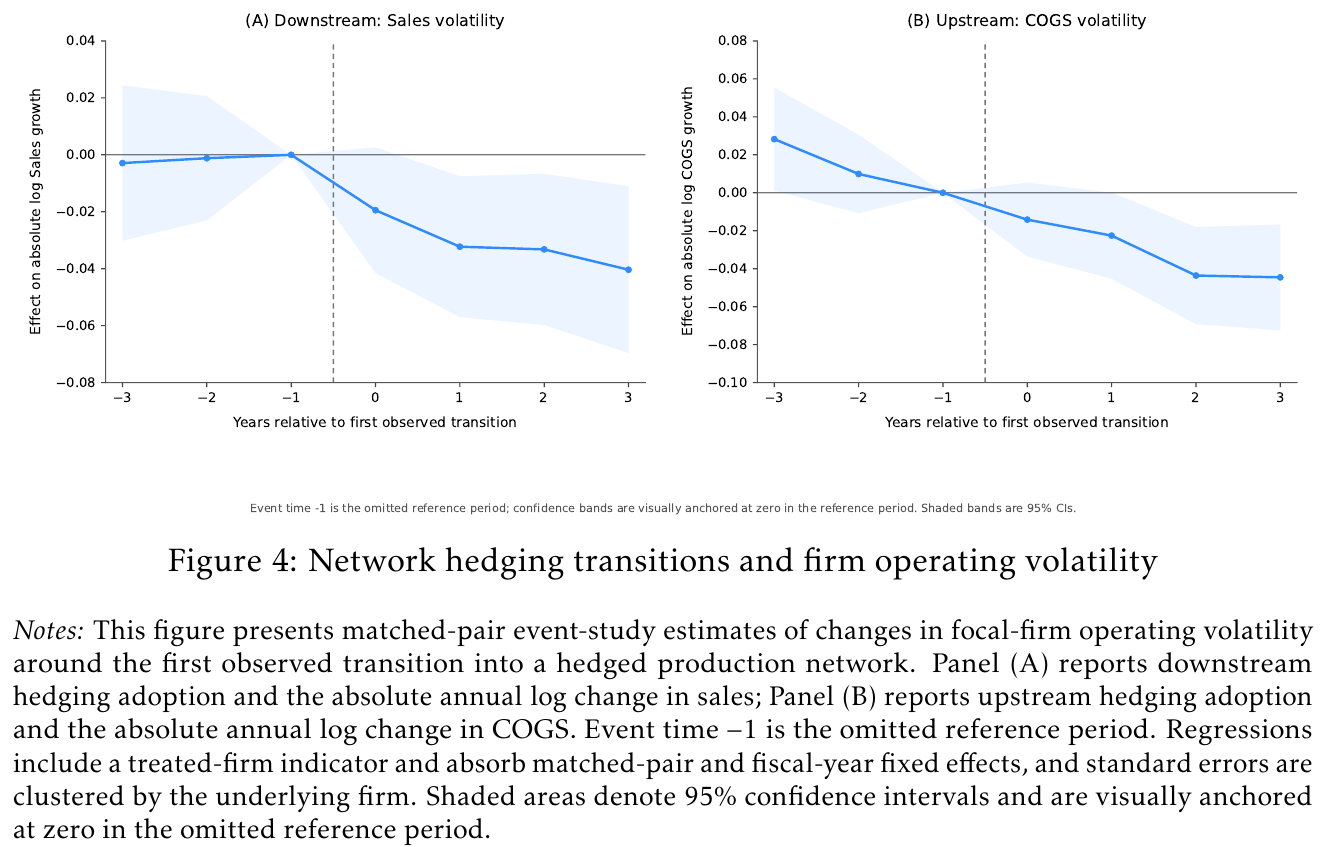
The dynamics are suggestive in the right way: the decline grows over time, from about −0.02 in year 0 to −0.04 by year +3 on the sales side, and from about −0.014 to −0.044 on the cogs side, with the earliest post coefficients’ bands including zero. The pre-period is mostly quiet, though the upstream coefficient at −3 is individually positive and significant (about +0.028), which is why that pre-trend p-value is 0.122 and not something more comfortable. The robustness battery is long and uneventful in the good sense: controlling for own hedging, lagged own hedging, firm-specific realized currency volatility, link churn, persistence of the network-hedging indicator and different matching weights, the estimates range from −0.027 to −0.048, all significant at 5%, and adding a control never moves the number by more than 0.002.

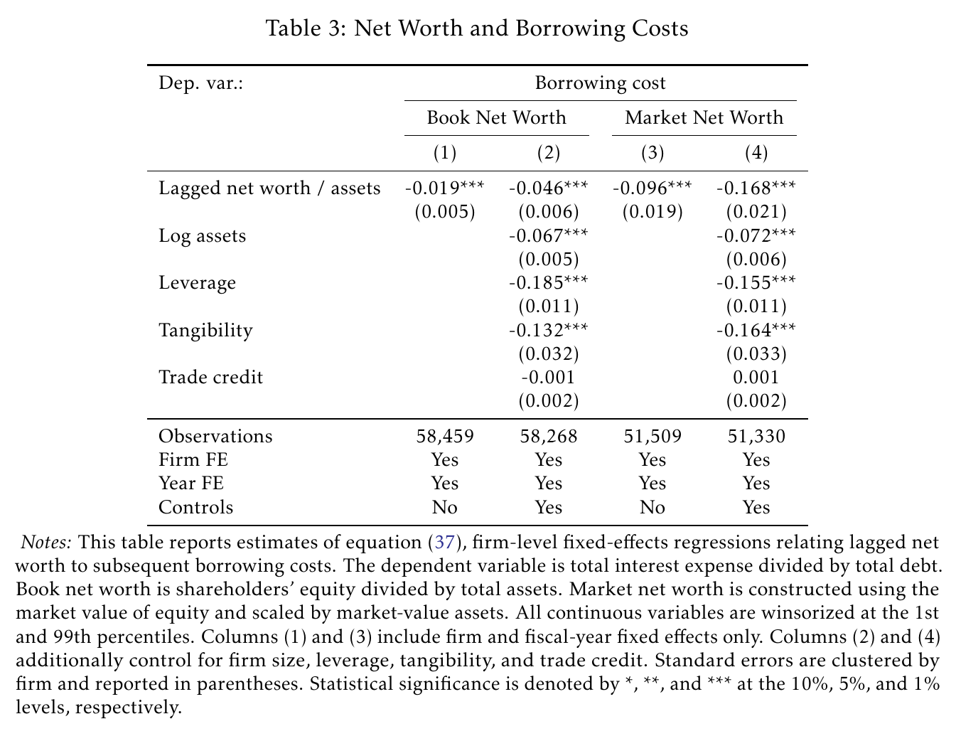
The mechanism evidence is more associational. Firms with higher lagged net worth pay lower interest expense per dollar of debt: 10 points more book net worth over assets goes with a 0.46 point lower rate, and 10 points more market net worth with a 1.7 point lower rate, with firm and year fixed effects. That is the credit schedule, more or less, seen in the data, though nobody is claiming it is causal.

The calibration, and the one surprising thing

Chen then puts the model on the 2022 bea input-output accounts, 60 industries, five equally likely annual dollar states drawn from the Fed’s broad index, and an annual preset-price share of 0.179. The price-risk and demand-risk channels run in two separate economies, an import-price one and a foreign-demand one; nobody faces both at once. The only internally calibrated parameter is $\gamma$, set to 7.6533 so that aggregate notional over gross output matches 3.56% in fiscal 2022 (an upper bound, since reported derivatives also hedge financing and translation exposure). The untargeted cross-sector fit is decent, with a Spearman correlation of 0.83 across 16 sectors, though the model spreads hedging too evenly: durables hedge more in the data than in the model, and mining and agriculture much less.

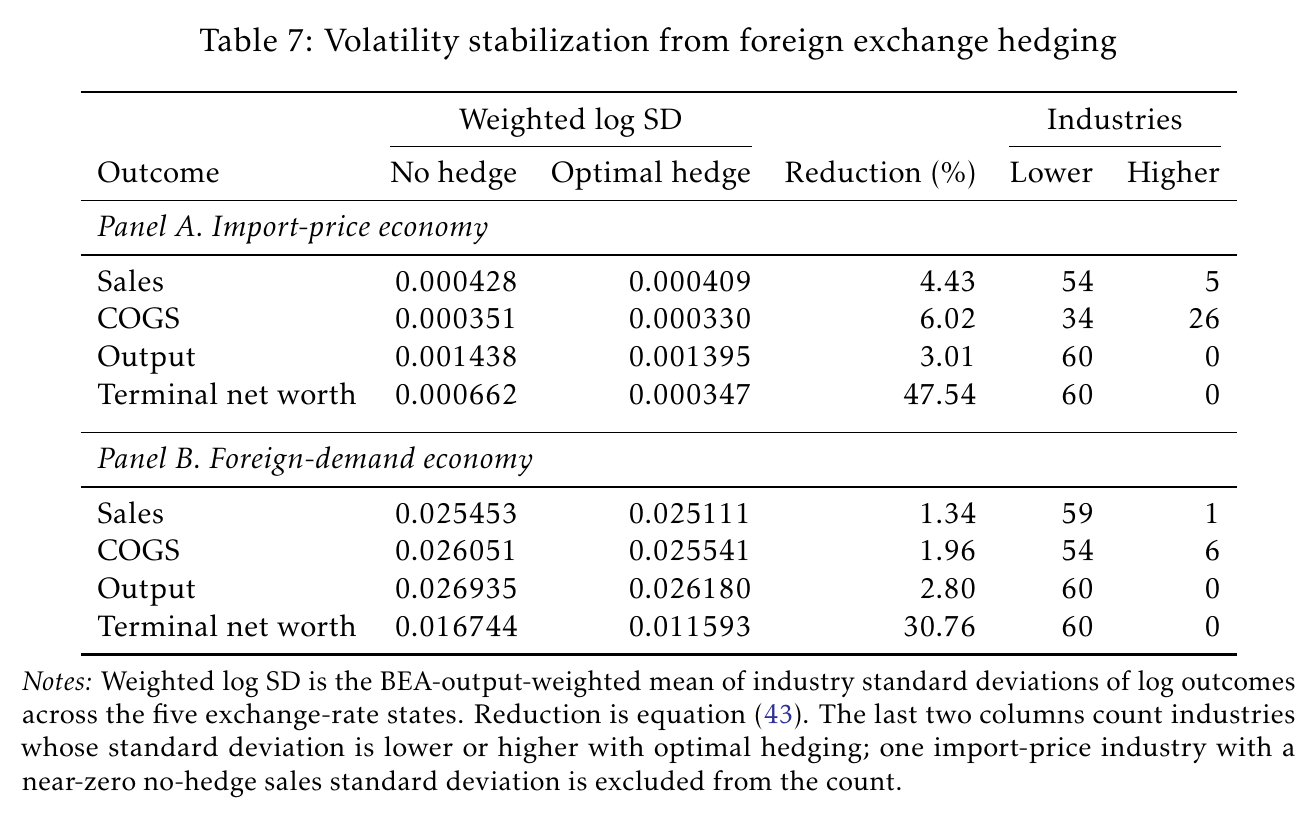
Giving firms access to hedging, relative to no hedging, cuts terminal net-worth volatility by 47.5% in the import-price economy and 30.8% in the foreign-demand economy. Operating volatility falls much less: output by 3.0% and 2.8%, sales by 4.4% and 1.3%, cogs by 6.0% and 2.0%. So hedging is mostly a financial stabilizer, which is what you’d expect from a friction that lives on the price of credit. (cogs volatility actually rises in 26 industries in the import economy and 6 in the demand economy: if you keep producing in the expensive-input states, your input bill varies more, even though your input prices are steadier.)

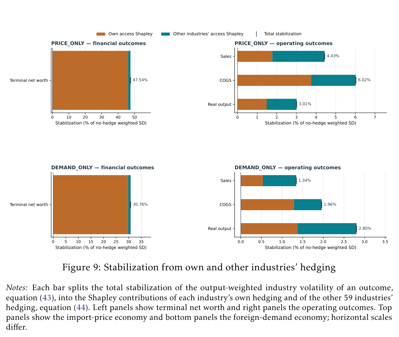
Here is the interesting part. Split each industry’s stabilization, Shapley-style, into the bit from its own hedge and the bit from everyone else’s. For net worth, about 97% is your own hedge, which is unsurprising, because the derivative pays you. For the real side, a large share comes from other industries: about half of output stabilization (50.5% and 51.0%), about 60% of sales stabilization, and 34–38% of cogs stabilization. With your own hedge switched off, everyone else’s hedging alone cuts your output volatility by about half of what all hedging does. The logic is in the model: a rigid-price firm meeting fixed demand doesn’t change its production when its bank account gets bigger, and a flexible-price firm changes it only through its price; but your supplier sector’s hedge changes the price you pay, and your customer sector’s hedge changes your orders. That rigid-price case is the paper’s illustration, not a claim that your own hedge doesn’t matter for output; it still supplies about half. But the punchline stands: hedging is “a private stabilizer of financial positions and a network stabilizer of real activity,” in the abstract’s phrase. A meaningful part of your operating stability is provided by people who don’t count your benefit when they choose how much of it to buy.

Two honest qualifications. These shares divide a small pie: total operating stabilization is 1–6%, and expected output barely moves (hedging raises expected real value added by something like 0.0001%). Hedging moves production across states; it doesn’t create more of it. And there is a gap between the empirical and quantitative magnitudes that the paper doesn’t close. The event study finds a 12–14% drop in a firm’s operating volatility when its first observed counterparty starts hedging; the model says all hedging, everywhere, lowers operating volatility by 1–6%. The paper says the Shapley “others” margin “is the margin that the event study measures” (p. 4), but never reconciles the sizes. Selection into hedged networks, an outcome measure that includes non-currency volatility, and a deliberately low-friction calibration are all candidates; the reader is left to pick.

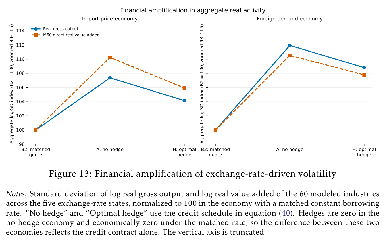
The cleanest way to see what hedging is for is Figure 13. Compare the baseline to an economy where every industry pays its baseline average rate in every state. The net-worth-dependent credit schedule raises aggregate value-added volatility by about 10% (10.2% and 10.5%). With optimal hedging, about 5.9% and 7.8% of extra volatility remains, so hedging offsets 42% and 26% of the amplification, “one-quarter to two-fifths.” That is an offset of the volatility finance adds, not of currency-driven volatility in total. Hedging, in this model, undoes some of the damage done by the credit market’s habit of charging you more exactly when you look worst. Single-industry removals tell a related story: knocking out one industry’s hedge has outside effects whose size lines up with supplier centrality (Spearman 0.72 and 0.83), with chemicals the standout, but no single industry moves aggregate volatility by more than a few hundredths of a percent.

What the room asked in 2025

The January 2025 talk drew three questions from the audience (the speakers are not identifiable from the recording). The first was simply how firms report hedging. Chen explained that the 10-K risk section describes currency, credit and interest-rate exposure and the instruments used, with fair values and usually the notional, adding that most, not all, firms report it. The 2026 draft documents the collection in an appendix and keeps missing values as missing rather than zero, but the selection question, which firms choose to disclose, is still there.

The second was the sharpest, and came in two parts. One: why the exchange rate moves matters; a dollar depreciation because the rest of the world is booming is a different event from one caused by U.S. policy. Chen agreed, said the model treats the rate as exogenous and that the identifying swings were monetary-policy driven, and called the fundamentals question “another research paper.” The 2026 draft still uses an exogenous common dollar factor. Two: even under dominant-currency pricing, demand depends on exchange rates and on demand elasticities, and a firm like Intel faces demand risk it has no market to hedge. Chen pivoted to operational hedging and said the paper studies exposure after operational hedging; the questioner offered to take it offline. The spanning point, that a currency forward is a crude instrument against a demand curve, was left mostly unanswered. The 2026 model separates the foreign demand elasticity to the exchange rate from the price elasticity and is candid that the forward supplies one risky payoff pattern, not complete contingent claims; that is an acknowledgement, not a solution.

The third: the network regressions assume independent errors when the whole argument is that firms are linked. Chen said lagged regressors partly addressed it and that those regressions were descriptive. In 2026 the allocation regressions still use firm-clustered standard errors and are still framed descriptively, and the causal weight sits on the event study, which is a reasonable division of labor.

What changed between 2025 and 2026

Quite a lot, and mostly in the direction of saying less with more support. The paper went from coauthored to solo and gained “Spillovers” in its title; the draft gives no reason, and nothing suggests the audience caused any particular change.

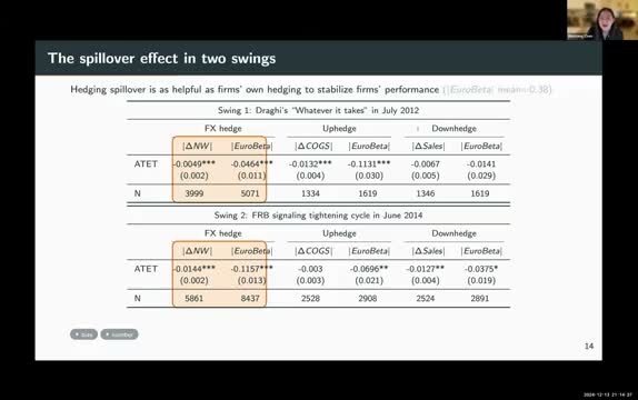
The identification was rebuilt. In 2025 it rested on propensity-score matching of euro-exposed firms around two eur/usd swings, Draghi’s “whatever it takes” in 2012 and the Fed’s tightening signal in 2014, with network hedging measured as a weighted probability over three layers of suppliers and customers and an extra outcome, a “euro beta” from factor regressions. The headline was that upstream hedging went with 1.32% smaller cogs fluctuations and downstream hedging with 1.27% smaller sales volatility, and the slide shows several insignificant cells. The 2026 draft throws all of that out for the first-adoption event study over 2003–2019, with pre-trend tests and the robustness battery, and the euro beta is gone.

The strategic-interaction claim was dropped. In 2025 Chen reported that firms hedge less when connected firms hedge more (the talk said “strategic complementarities” while describing substitutes): about −$0.161 million per 10% more upstream hedging and −$0.083 million downstream. The 2026 draft says spillovers “do not by themselves establish strategic complementarities in hedging or a welfare inefficiency,” and the allocation fact is now the opposite-sounding one that firms with more customers and suppliers hedge more, presented descriptively.

The model grew up: three dates instead of two, preset dollar prices, a rate indexed to projected net worth rather than an exogenous net-worth constraint, the separation of optimal from stabilizing hedges (Props 3–4) and the exporter condition (A9). The calibration went from 71 sectors grouped into five, matched to two sectoral hedging ratios, to 60 bea industries with a single target.

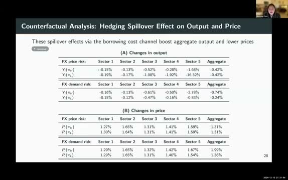
And the headline changed from levels to volatility. In 2025, shutting the borrowing-rate channel cut output and raised prices; the slide shows output down 0.24% to 0.74% and prices up 1.31% to 1.99% (the spoken numbers, about 0.9% and 1.5%, don’t quite match the slide). The 2026 analogue, the matched-constant-rate comparison, runs in the same direction but smaller: baseline expected value added is 0.20–0.22% higher than under the matched rate, and the paper explicitly calls that “not an estimate of the output gain from hedging,” which is the near-zero number. So the 2025 “hedging boosts output and lowers prices” story was not reversed so much as re-scoped into what it always more plausibly was, a story about the second moment. The policy talk followed suit: 2025’s worries about midstream overhedging, “market research” subsidies and U.S. firms as “global insurance providers” give way to an open question on efficiency and a narrower implication from the calibrated removals, that disruptions to the supply of hedging “may propagate” beyond the firms that lose access, most of all when central suppliers are hit.

Which leaves you with a pleasingly odd picture of what a currency forward is for. The cfo buys it to keep the bank happy, and it does that. But a good part of what it does for the real economy shows up on other people’s income statements, in the form of input prices that wobble a little less and orders that arrive a little more reliably, and none of those people sent a thank-you note, because none of them knew.

What Verdelhan asked in 2026

The nber talk was essentially the October draft presented, so the headline numbers are where this note left them, and the slide keeps the text’s modest “~60% of sales” rather than the bars (07:03:56). The one addition is a reason for the two separate economies: Chen said that while hand-collecting the filings she saw firms use separate contracts for price risk and demand risk, because maturities and currencies differ, so the two don’t simply net (07:11:50; the captions are rough here, so that is a paraphrase).

The floor did its audible work during the talk. One questioner pressed the gap between trade-literature price elasticities and the elasticity of demand to the exchange rate, a cousin of the 2025 objection; Chen said she calibrates by sector from the literature and isn’t trying to match that (07:14:11). Another asked about unobservable reasons for adoption; she agreed there can be confounders and said she controls for as much as she can (07:36:15). When the Shapley slide said half of output stabilization, someone pointed out that this was half of something very small, and Chen agreed (07:44:56). And someone asked whether a firm’s borrowing cost falls when it starts to hedge, and whether she had evidence. Yes, she said, she would show it (07:30:15). Hold that thought.

Adrien Verdelhan called it a very good paper on a literature that needs one, since firms don’t have to report the details of their hedging. Then the discussant shrank the model to one firm and tried to rebuild the data.

Take one importer with rigid prices. After a depreciation its bill is bigger and its net worth lower, so a dollar is worth more in that state and the importer always buys foreign currency forward (07:54:57). This is unambiguous and, for Chen’s purposes, useless: with price and output fixed, nothing propagates. So she needs flexible prices, and they bring a second force. The depreciation raises your price, demand falls, you buy less, and the bill shrinks in exactly the state where you wanted the dollar. The importer now hedges the conventional way only if $\gamma\times\text{margin}>1$, which at $\gamma=7.65$ means an operating margin above 13% (07:57:20). The slide calls this the same condition as (A9) for the exporter, so the paper’s awkward case is also the importer’s case, in the only version of the model where anything spills over. Timing is load-bearing too: set the rate at date 0 on expected net worth, and a fair forward wouldn’t change it (07:55:41).

Next came numbers on the credit schedule, which Verdelhan mostly liked. A firm 20 points of revenue below its reference pays 11.19%, one 10 points above pays 3.92%, and the slope, 13.4 basis points per point, sits between the 4.6 and 16.8 implied by Table 3, if assets are about revenue (07:58:30). But firms barely travel along that curve. Across currency states the standard deviation of borrowing rates without hedging is 0.35 basis points in the import-price economy and 9.7 in the foreign-demand economy, and hedging takes those to 0.19 and 7.0. That is the movement the network channel has to work with. Then came the part the discussant said was harder to swallow than the mechanism: “Why does the borrowing rate depend on net worth, since the firm never defaults?” (07:58:48). An earlier slide of the discussant’s offers the charitable reading, that the schedule stands in for a convex cost of external finance as in Froot, Scharfstein and Stein (1993) (07:54:00). It is still a lender charging for a risk the model has promised isn’t there.

The replication is automated: a 10-K text screen over fiscal 2000–2025, plus notionals tagged in xbrl from fiscal 2011 (08:00:30). The aggregate works beautifully, $1.22 trillion for fiscal 2022 against the $1.25 trillion implied by the calibration target, and the extensive margin gives the same shape at lower levels. It also argues for Chen’s labor: in 1,000 10-Ks filed in 2015, half of the firms the text screen flags have no tagged notional, many of them genuine hedgers. One worry is that first-time disclosure spikes in fiscal 2009, when fas 161 required the numbers (08:01:20), so a first adoption may be a first report, and later calm may look like a spillover. Verdelhan granted that the draft’s control for realized currency volatility addresses this.

’)

The bigger worry is that the intensive margin does not replicate. Chen’s bars run past 80% of sales; Verdelhan’s mean stays below about 17% and even the top decile reaches only 21–39%. “What am I missing?” the slide asks. This note told you earlier to trust the chart over the text. That was a ruling on which number describes the paper; whether either describes the firms is now open. (One thing Verdelhan didn’t raise: Chen’s own slide puts average notional among hedgers at 7.7% of assets (07:32:03). The denominator differs and that figure is winsorized, so it is only a hint, but it sits much nearer Verdelhan’s line than Chen’s bars.) The discussant also noted that a notional doesn’t say what it hedges, and suspects much of it is swaps on foreign-currency debt (08:03:10), which a hand-collected dataset could actually separate.

Then the thought you were holding. Verdelhan went back to the questioner from 07:30, whose name neither transcript catches, and listed what Chen had shown instead: hedging goes with lower volatility of sales and net worth, and net worth in levels goes with lower borrowing costs, “but no direct link between fx hedging and borrowing costs” (08:03:45). So test that, Verdelhan said, and test the 13% condition: does the hedge sign flip for low-margin firms? (That one needs a direction that the draft’s notional totals don’t record.)

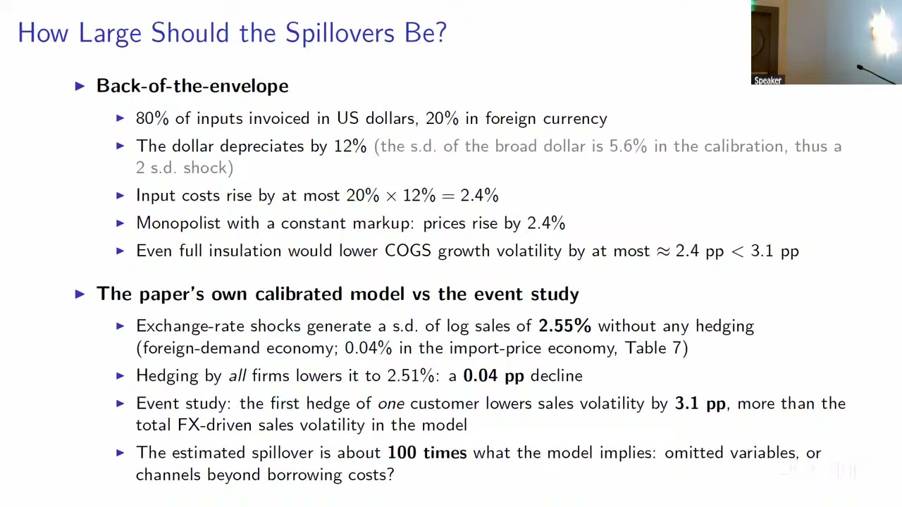
The hardest slide came last and time ran out; “let’s skip this,” Verdelhan said (08:04:23). It is worth pausing on. In the calibrated foreign-demand economy, currency shocks generate a log-sales standard deviation of 2.55% with no hedging at all (0.04% in the import-price one), and hedging by every firm takes it to 2.51%. The event study says the first hedge of one customer does 3.1 points, more than all the currency-driven sales volatility in the model. Table 7’s unrounded figures give a ratio nearer 90 than 100, and the objects differ, since the event study’s outcome is any absolute sales growth; that is the slide’s “omitted variables” option. But this note put the gap as 12–14% against 1–6%, and in levels it looks a good deal worse.

About four minutes of open discussion follow, but the room audio barely registers, and neither the captions nor two Whisper passes yield a sentence I would attribute to anyone; there is no audible reply from Chen on the recording. Verdelhan’s last slide says “Highly recommended reading!” and the recommendation was clearly meant. The previous section ended with firms that never sent a thank-you note for their steadier input prices. Verdelhan’s arithmetic raises the question of who it should be addressed to.

References