Can Sticky Price Models Generate Volatile and Persistent Real Exchange Rates?

V. V. Chari, Patrick Kehoe and Ellen McGrattan, Review of Economic Studies 2002. Read here in the Minneapolis Fed Staff Report 277 version (revised July 2002). No talk recording exists; written from the paper alone.

The title is a question, and the paper’s honest answer is: yes on volatility, almost on persistence, and in the process we discovered something worse. This is the definitive stress test of the profession’s favorite story about exchange rates — Dornbusch’s 1976 idea that monetary shocks interacting with sticky prices produce the big swings — performed by three authors with impeccable flexible-price credentials, which is part of why the verdict carried weight. They build the best sticky-price open-economy model 2002 could assemble and push it until it breaks, and the location of the break turned out to matter more than the test.

First, aim the model at the right target

Before the model, a measurement result that redirected the literature. Real exchange rate movements can come from two places: deviations from the law of one price for traded goods, or movements in the relative price of nontraded to traded goods (the classic Balassa–Samuelson channel that Backus–Smith, earlier in this list, leaned on). Decomposing U.S.–Europe data 1973–1998, CKM find the nontraded-goods component explains at most 2 percent of real exchange rate variance (their decomposition: 3.64 = 4.10 + 0.076 − 0.54, so 0.076/3.64). Echoing Engel’s work, virtually all the action is in traded-goods prices failing to be equalized across borders. So the model drops nontraded goods entirely and generates real exchange rate movements purely from pricing-to-market: monopolistic intermediate-goods firms with exclusive national distribution rights (no arbitrage between markets — the Coca-Cola clause from Obstfeld–Rogoff’s paper, formalized) set prices separately in each country’s currency, in advance, staggered, fixed for N = 4 quarters.

The volatility answer: yes, if you buy σ = 5

With complete asset markets, the model has one load-bearing equation — the real exchange rate is proportional to the ratio of marginal utilities of consumption:

(equation 14 in the paper). Log-linearized with separable preferences, this delivers std(q̂) ≈ σ · std(ĉ − ĉ*): the volatility of the real exchange rate is risk aversion times the volatility of relative consumption. To make the exchange rate 4.36 times as volatile as output — the data — you need σ ≈ 5. And it works: the benchmark produces relative volatilities of 4.32 (nominal) and 4.27 (real) against 4.67 and 4.36 in the data, with monetary shocks sized to match output volatility. Persistence comes out at 0.62 against 0.83 — respectable, but short; they name it the persistence anomaly, show it is inherited one-for-one from the autocorrelation of consumption, and report with some chagrin that sticky wages, the natural fix, “does little.” (Their closing wish — a mechanism generating endogenous stickiness from small frictions — reads as a to-do list for the following two decades of macro.)

So the Dornbusch story survives, at a price: exogenous year-long price fixity, high risk aversion, and preferences separable in leisure (the nonseparable variant collapses exchange-rate volatility — see the model comparison table below).

The break: an anomaly that sticky prices cannot touch

Then the trap springs. Equation (14) does not merely set the exchange rate’s volatility; it welds the exchange rate to relative consumption with correlation one. In the data, that correlation — the Backus–Smith correlation, from paper five of this reading list — is −0.35 for the U.S. against Europe. Model: +1.00. Data: −0.35.

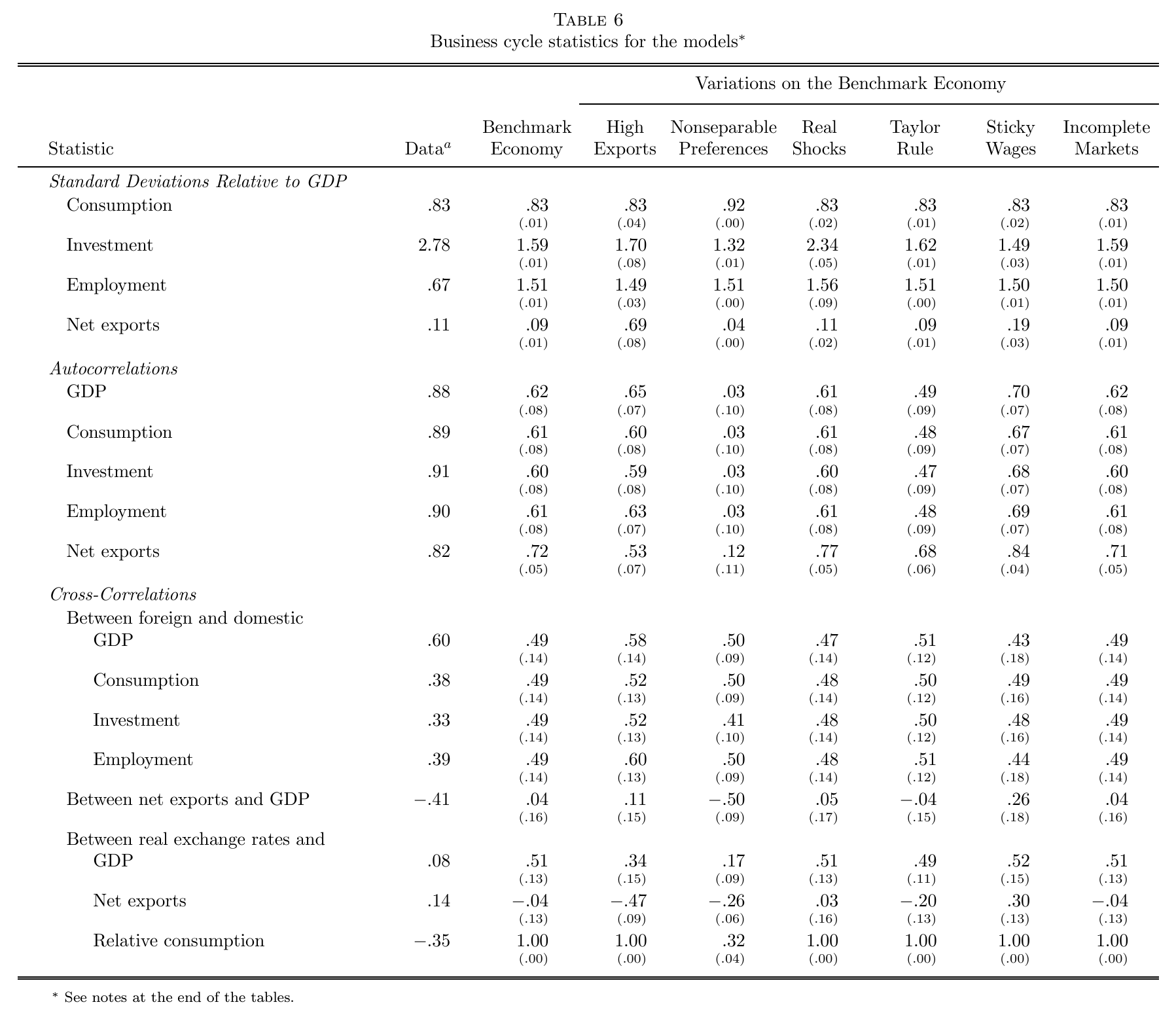
What makes this the paper’s lasting contribution is the demonstration of how deep the failure runs. The proportionality (14) follows from complete markets alone — “regardless of the frictions in the goods and labor markets like sticky prices, sticky wages, shipping costs, and so on.” Fine, so break the asset market: replace complete markets with a single uncontingent nominal bond, the workhorse incompleteness of the entire literature. The correlation stays at 1.00 — the bond economy tracks the complete-markets allocation too closely for the difference to matter. Habit persistence, the fix-all of late-90s asset pricing? Their back-of-envelope calculations say it won’t shrink the anomaly either. The conclusion is written as a warning to the field: essentially every model in the international business cycle literature, real or nominal, has one of these two asset structures, so essentially every model has this anomaly, and fixing it “should focus on incorporating richer forms of asset market frictions.”

Scorecard details worth keeping

The sensitivity analysis contains several honest confessions with long shelf lives. Employment in the model is 1.51 times as volatile as output against 0.67 in the data — a structural feature of sticky-price models, since with output demand-determined and capital fixed, ŷ ≈ (1−α)·l̂ forces labor to be more volatile than output, and makes measured productivity countercyclical (it is procyclical in the data). Investment is half as volatile as it should be, because matching consumption volatility at σ = 5 requires stiff adjustment costs. The price ratio is four times too volatile, so nominal and real exchange rates correlate at 0.76 instead of the data’s 0.99. Raising trade openness from the U.S.–Europe bilateral 1.6 percent to 15 percent changes little. None of these is fatal; together they define the model’s frontier.

The paper’s position in this reading list is that of the pivot. It closes the arc that started with BKK — the same Patrick Kehoe, note, testing the nominal-frictions repair of the real model he co-built a decade earlier — and it hands the baton forward twice: the 2 percent decomposition and the pricing-to-market machinery feed directly into Burstein–Gopinath’s handbook chapter (next), while the verdict that goods-market frictions cannot break the consumption–exchange-rate link is precisely the opening claimed by Itskhoki–Mukhin’s segmented financial market (previous entry), where the “richer asset market friction” CKM requisitioned finally reports for duty. Twenty years on, their closing sentence looks less like a confession of failure than a purchase order that took two decades to fill.