Notes on:

Diversification through Trade

Francesco Caselli, Miklós Koren, Milan Lisicky & Silvana Tenreyro
The Quarterly Journal of Economics 135(1), 2020, 449-502
2020
international trade · macroeconomic volatility · diversification · quantitative trade models · business cycles
doi
Opus 5 (reading, diagram and writing)

Francesco Caselli, Miklós Koren, Milan Lisicky and Silvana Tenreyro, “Diversification through Trade,” Quarterly Journal of Economics 135(1), 2020, 449–502; advance access 19 September 2019. This digest is from the paper — the published QJE version. There was no talk and no discussant.

The standard worry about trade and volatility is a portfolio worry that forgot it was one. You are a country. You open to trade, you specialize into the few things you are relatively good at, and your income now rides on those few things. Newbery and Stiglitz said roughly this in 1984, and by 2011 it had hardened into a trade-off a development ministry could write down: trade buys you productivity, you pay in wobble. This paper points out two holes, both of the kind you find by taking the portfolio analogy literally rather than loosely.

Hole one: concentration only hurts if the risk is asset-specific. If most of the variance in national income comes from shocks hitting every sector at once, the composition of your basket is beside the point: the holdings are correlated by construction. The evidence says country-wide shocks are at least as important as sectoral ones (p. 450). Hole two: a concentrated portfolio is not mechanically riskier. It depends what you concentrated into, and how that covaries with your own national shock.

Which makes the contribution obvious in retrospect, the good kind of obvious. If your problem is a shock to the whole country, then trade is diversification: an open economy sells into world demand and buys from world supply, so a bad domestic draw is partly absorbed by everyone else’s good draw. That channel runs opposite in sign to specialization, and the job is to say which is bigger.

The model

Schematic (ours, not an exhibit from the paper): the within-period timing that makes both channels exist — factor markets clear before the shock, goods markets after it. Open the figure in a new tab

Underneath is a stochastic Eaton–Kortum: 25 economies, 24 sectors, 1972–2007, with a full input–output matrix so every sector buys intermediates from every other (pp. 451, 455, 464). The load-bearing assumption is timing. Equipped labour goes to sectors before shocks are realized, by

\frac{L^{j}_{nt}}{L_{nt}} = E_{t-1}\!\left[\frac{w^{j}_{nt}L^{j}_{nt}}{\sum_k w^{k}_{nt}L^{k}_{nt}}\right],\qquad \forall j,t,

where $L^{j}_{nt}$ is labour in sector $j$ of country $n$ and $w^{j}_{nt}$ its wage: each sector gets its expected share of the wage bill (equation 12, p. 460). Then shocks land, and then producers buy each input from the cheapest supplier on earth. Goods markets adjust ex post; factor markets do not — deliberately, since without the rigidity labour would walk out of the unlucky sector and the specialization channel “could not arise” at all (pp. 456–457).

The intuition comes from a one-sector case. Under autarky,

Var(\hat Y_{nt}) = \frac{1}{(\beta\theta)^{2}}\,Var(\hat Z_{nt}),

with $\hat Y$ and $\hat Z$ the detrended logs of real income and productivity, $\beta$ the labour share, $\theta$ the Fréchet shape parameter (p. 462). Under costless trade,

Var(\hat Y_{nt}) = \left(\frac{1}{\beta\theta}\right)^{2}\left\{\begin{array}{c}\left(\frac{\gamma_n+\beta\theta}{1+\beta\theta}\right)^{2} Var(\hat Z_{nt}) + \left[\frac{1}{1+\beta\theta}\right]^{2}\sum_{m\neq i}\gamma_m^{2}\,Var(\hat Z_{mt})\\[4pt] + \,2\,\frac{\gamma_n+\beta\theta}{1+\beta\theta}\,\frac{1}{1+\beta\theta}\sum_{m\neq n}\gamma_m\,Cov(\hat Z_m,\hat Z_n)\end{array}\right\},

where $\gamma_m$ is partner $m$ ’s relative size, so the own-shock loading drops below one while foreign variances and covariances enter for the first time (p. 462; the printed $m\neq i$ on the middle sum looks like a typesetting slip for $m\neq n$ ). That is the whole theory. Your own shock gets a smaller weight, the more so the smaller you are, but you inherit your partners’. You lose if they are big, volatile, or move with you.

What the numbers say

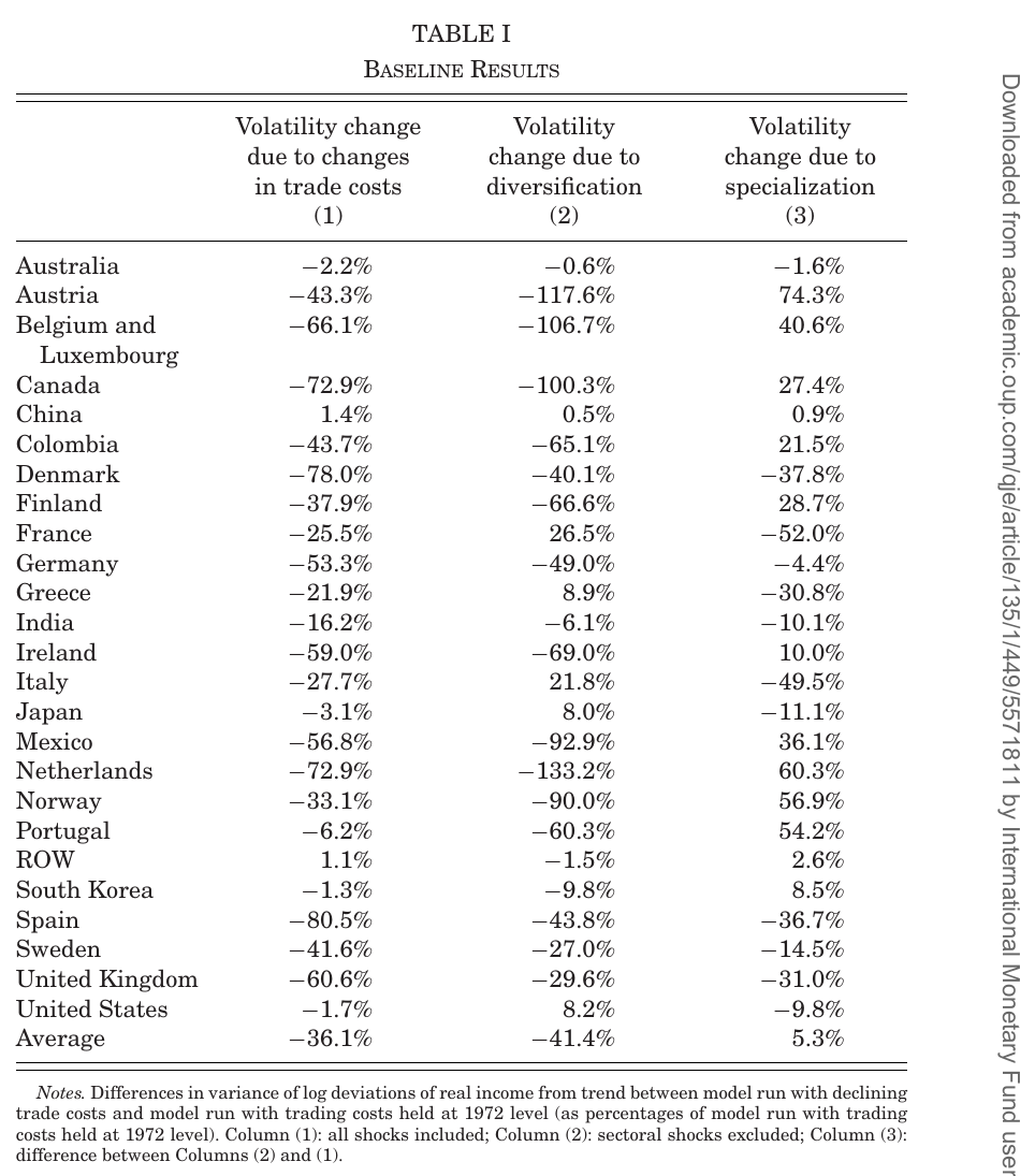
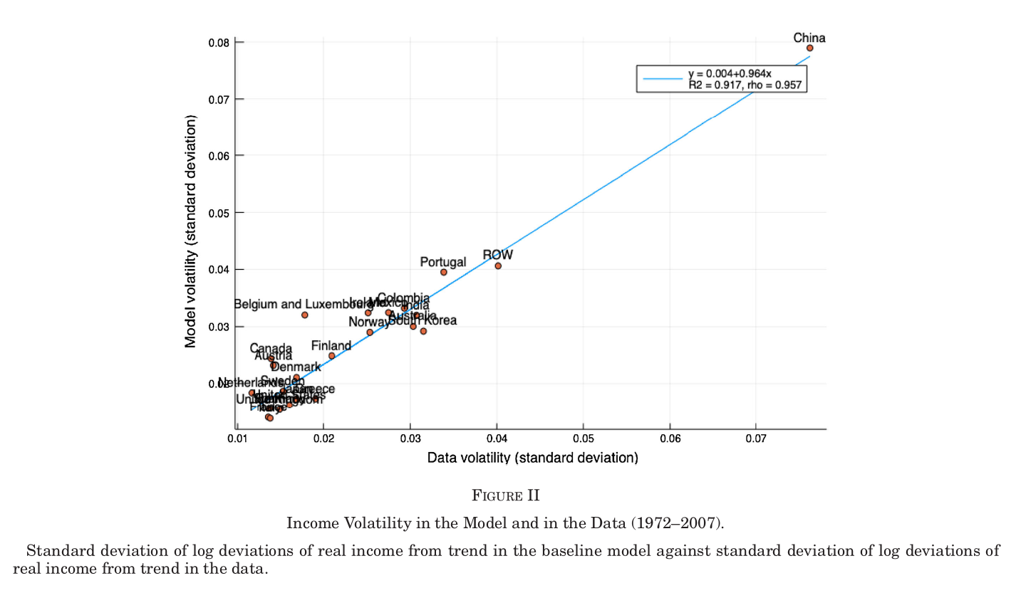
Three-column table of 25 countries plus an average row, showing the percentage change in income variance caused by falling trade costs, split into a diversification column and a specialization column; the average row reads minus 36.1 percent, minus 41.4 percent, plus 5.3 percent. — Table I, paper p. 473: “Baseline Results” — column (1) is the total effect of the observed fall in trade costs on income variance, column (2) the country-diversification channel alone, column (3) = (1) − (2) the sectoral-specialization residual.

The counterfactual is not autarky but a world where trade costs stayed at 1972 levels. Against that, the average country’s income variance is 36.1% lower: −41.4 points diversification, +5.3 points specialization, the nice channel about eight times the nasty one (p. 475). Trade raised volatility in two of 25 rows, by 1.4% and 1.1%. Nine countries came in more than 50% below, Spain lowest at −80.5%. One reading trap: every entry is divided by the same denominator, the full 1972-cost variance, including the column run with sectoral shocks off — a common yardstick chosen so column (3) is exactly column (1) minus column (2), which is why the Netherlands can post −133.2% without anything having fallen by more than all of it. The licence for the whole exercise is fit: model and data standard deviations correlate at 0.96, or 0.88 without China.

Scatter of model-implied against actual standard deviation of detrended real income for 25 labelled countries, hugging a fitted line y = 0.004 + 0.964x with R-squared 0.917; China sits alone at the top right near 0.08. — Figure II, paper p. 472: “Income Volatility in the Model and in the Data (1972–2007)” — correlation 0.96 for the standard deviation, 0.88 once China is dropped.

Same three-column country table as Table I but for a model with no intermediate inputs; every entry is an order of magnitude smaller and the average row reads minus 3.5 percent, minus 7.0 percent, plus 3.5 percent. — Table VII, paper p. 486: “Role of Input-Output Linkages” — with γ^{kj} = 0 the whole effect of trade on volatility shrinks from −36.1% to −3.5%, so intermediate sourcing is the pipe the diversification runs through.

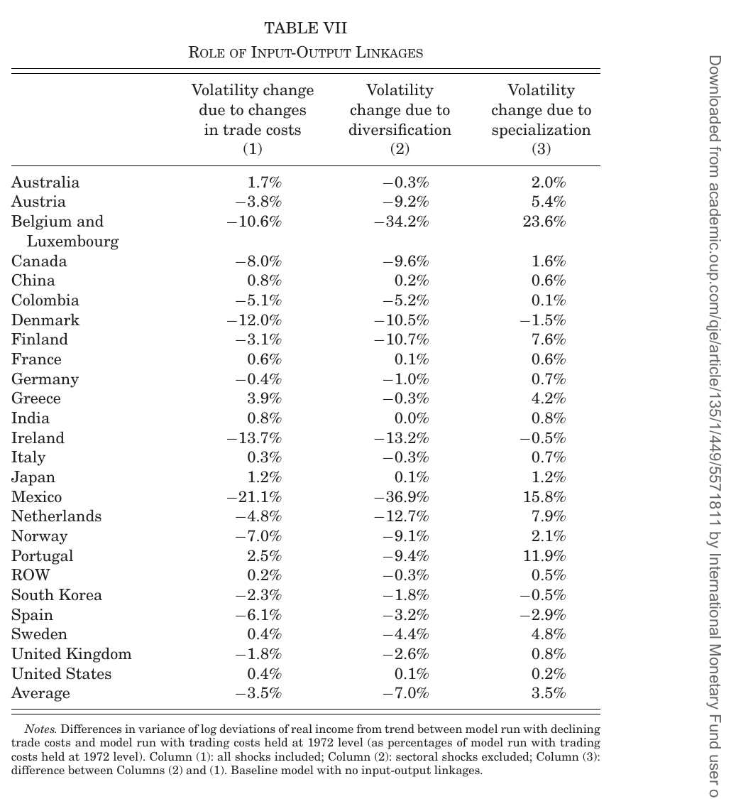
The plumbing matters enormously. Set every intermediate share to zero and rerun, and the average effect collapses to −3.5%: “allowing firms to source inputs from other sectors is crucial to capture the full effects of trade on volatility” (p. 487). Diversification arrives less as export demand than through the input matrix.

The surprising part

In France, both channels run backwards. Diversification raises volatility by 26.5% and specialization lowers it by 52.0%; Italy is 21.8% and −49.5%. Both signs flipped in two large economies, and the net effect is still a fall: trade stabilized them for precisely the reason everyone worried about. More generally the specialization channel — the basis for four decades of “trade makes you volatile” — has the wrong sign in 12 of 25 countries, because many were “pushed to specialize into less volatile sectors or into sectors that comove negatively” with their own aggregate shock (p. 475). Specialization is not a risk. It is a portfolio choice, and on average countries chose reasonably.

What a critical reader would press on

Nobody said any of this; it is what the design invites. Trade costs are not measured but inverted out of a gravity equation under symmetry, and the authors concede the levels are “very large” and may absorb home bias (p. 465). Productivity is a residual of that residual. The country shock is defined as an expenditure-weighted within-country mean, and with services at 70–80% of value added, “country shock” is largely “services shock” — a nontraded sector whose diversification travels entirely through the input matrix. Magnitudes ride on $\theta$ : −52.6% at $\theta=2$ against −22.5% at $\theta=8$ (pp. 478–479). There are no standard errors anywhere. And the sample stops in 2007 because the model omits what caused the crisis (fn. 4, p. 451), which leaves outside the window the one episode that would most severely test a theory caveated on partners’ shocks moving with yours.

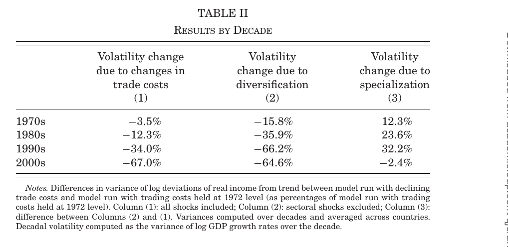
Four-row table by decade from the 1970s to the 2000s, showing the total volatility change growing from minus 3.5 percent to minus 67.0 percent while the specialization column turns from plus 12.3 percent to minus 2.4 percent. — Table II, paper p. 476: “Results by Decade” — the trade effect compounds steadily, but the diversification channel stops growing after the 1990s and the specialization channel changes sign in the 2000s.

The last row of that table is the one to sit with. The diversification dividend, having compounded for thirty years, stops growing in 2000–2007 — and the paper’s own formula names the suspect, which is the covariance term.