How Far Can Inclusion Go? The Long-term Impacts of Preferential College Admissions

Michela Carlana, Sara Chiuri, Enrico Miglino and Michela M. Tincani
Presented by Michela Carlana at the nber Economics of Talent Conference, Cambridge ma, 2 October 2026 (video). No discussant.
Paper version: cepr Discussion Paper 19128 (v. 2), dated July 2026 and revised 11 July 2026; the paper also circulates as nber Working Paper 32525. Where the talk and the paper give different numbers, the text says which one it is quoting.

A free option, valued by high-school seniors

A preferential admission offer is an option. You can take the reserved seat or leave it, and an option you are free to ignore cannot make you worse off. That is the result the paper builds on (Arcidiacono, Khan, and Vigdor 2011): an admission preference can hurt the student it targets only if there is a decision-making friction, such as a student who overestimates her chances of finishing the degree. So the mismatch hypothesis, which Sander (2004) put forward about American law schools and which the evidence on percent plans has mostly not supported, is really a claim that students misjudge what the option is worth. The holders are high-school seniors, and the paper’s main contribution is that it asked them, before they enrolled, what they thought their chances were.

The reason to look in Chile is that the existing evidence comes from students who were well prepared to begin with. The Texas Top Ten sample (Black, Denning and Rothstein 2023) sits at the 86th percentile of the relevant test distribution. pace’s targeted students sit at the 52nd percentile of Chile’s national grade-10 test, 0.9 sd below regular selective-college entrants, and 1.1 sd below them at the admission cutoff (paper pp. 2, 11). If mismatch shows up anywhere, it should show up here.

PACE, measured two ways

pace gives students in the top 15% of their school’s gpa ranking a reserved seat at one of Chile’s selective colleges. Only disadvantaged high schools take part, picked by a school vulnerability index. To use the seat a student must have attended the pace school in grades 11 and 12 and sat the psu entrance exam, although her score on it doesn’t count. The seats are supernumerary, so nobody admitted the regular way is displaced. The bundle also includes orientation sessions for everyone in the school and first-year tutoring that, Carlana said, almost nobody uses. The program went from 69 schools in 2014 to 456 by 2016.

The first design is an rct. In 2016 the government, on the team’s advice, randomly picked 64 of 218 eligible schools to join (the talk said 221; the paper drops three schools that had no target cohort). The sample is the 2,437 students who were in their school’s top 15% by grade 9–10 gpa before the announcement. The treatment is the whole pace-school package, including orientation and any change in effort while in school. That is broader than the admission offer itself, which only 54.2% of top-15% students in treated schools actually received (Carlana rounded it to 55%).

The second design is a fuzzy rdd at the 15% cutoff, using pace schools’ 2014–2016 cohorts, with equations (2) and (3) on paper p. 17:

Here $A_i$ is a pace admission offer, $p_{is}$ the policy’s gpa ranking score, $c_s$ the school’s cutoff (the lower of its 85th percentile and a national cutoff), $f$ and $g$ local linear functions that may differ on each side of the cutoff, $X_i$ controls, $\eta_s$ and $\nu_s$ school fixed effects, and $\delta$ the late for compliers. No one below the cutoff gets an offer and 85.36% of those just above do (the talk said 80%).

The outcomes are seven years of administrative education records and formal private-sector earnings from unemployment-insurance records. Earnings in years 8–15 are not observed. They are predicted with a surrogate index (Athey et al. 2026) trained on earlier graduates of the same schools. So “long-term” in the title means seven years observed and eight more forecast, and the forecast covers only formal private-sector work.

The top 15%: a reshuffle, not an expansion

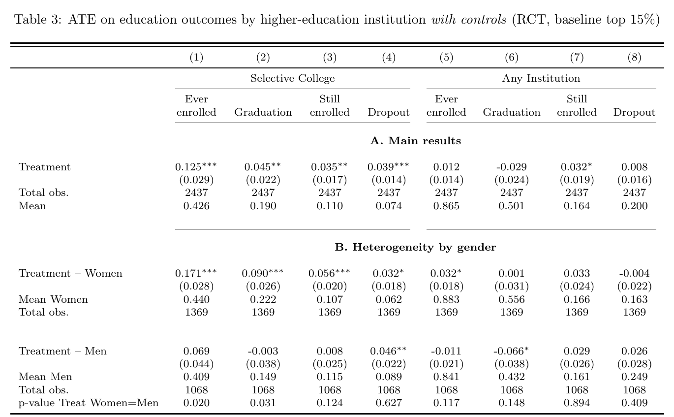
In the rct, being in a pace school raises selective-college enrollment by 12.5 percentage points on a control mean of 42.6% (29%), and selective-college graduation by 4.5 points on 19.0% (24%). Enrollment anywhere barely moves (+1.2, not significant) and neither does dropout from any institution (+0.8, not significant). So the policy works on the intensive margin. Students who would have gone to a vocational institute or a non-selective college go to a selective one instead, and a good share of them finish. The added margin at year 7 is students still enrolled without a degree (+3.2, significant at 10%), not students who have dropped out. In a literature where people mostly argue about whether these programs do harm, a program that does what it says is a respectable result.

The labor-market average is less impressive. Treated students earn 252 thousand pesos a year less over years 1–7, on a mean of 2,201 (about 11%), which is what happens when people are in harder programs for longer. After that nothing is significant, observed or predicted. The average student gets more degrees, a few lean years, and no detectable payoff.

Women take the option, men pay for it

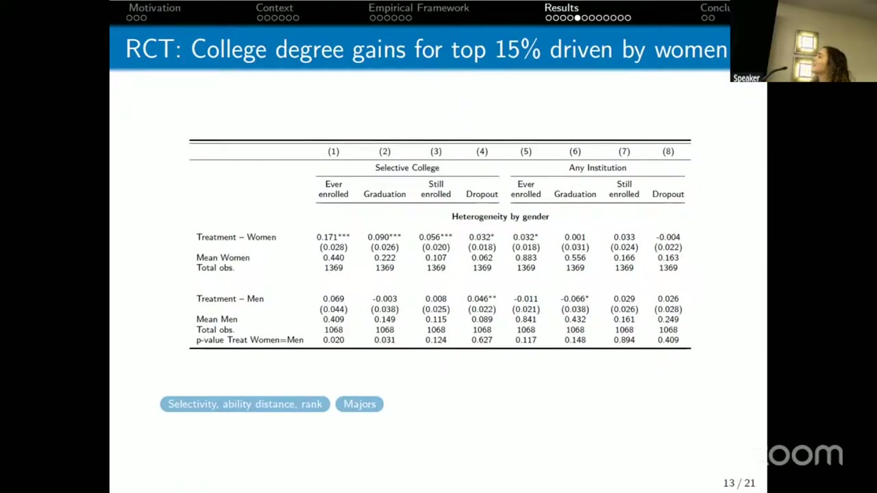
The average hides two opposite effects. Women’s selective enrollment rises 17.1 points and their selective graduation 9.0 points, on a control mean of 22.2%. Men’s selective graduation effect is −0.3 points. Carlana called this a “very precisely estimated zero”, which is generous: the standard error is 3.8 points, so the 95% interval runs from about −8 to +7. It is a zero, but not a precise one. Men’s selective dropout rises 4.6 points and their graduation from any institution falls 6.6 points (10% level) on a mean of 43.2%. The paper reads that as partly delay and partly lost degrees. The gender differences are significant for selective enrollment (p = 0.020) and selective graduation (p = 0.031).

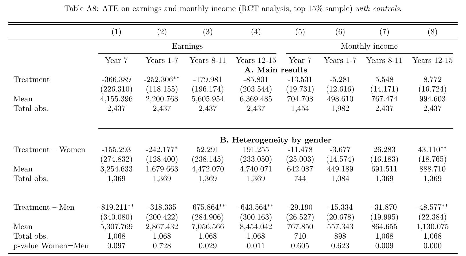
The earnings follow the degrees. Women lose 242 thousand pesos a year in years 1–7 on a mean of 1,680, the 14.4% Carlana quoted. Their predicted monthly income in years 12–15 then rises by 43.1 thousand on 888.7, about 5%. For men the predicted monthly income in years 12–15 falls by 48.6 on 1,130.1 (−4.3% by the table; the paper’s text says 4.4%). Carlana said men had “no significant short-term earnings impacts”. That is true for the years 1–7 average (−318, not significant), but men’s observed year-7 earnings fall by 819 thousand, significant at 5%.

Put together, the predicted gender gap in monthly income shrinks by 38%, from 241.4 thousand pesos to about 149.7. The paper writes “from 241.4 to 91.7”, but 91.7 is the size of the reduction, not the new gap; the 38% is right. Part of that narrowing comes from men losing ground, which is not how a program brochure would describe closing a gender gap.

At the margin: 1.15 dropouts per degree

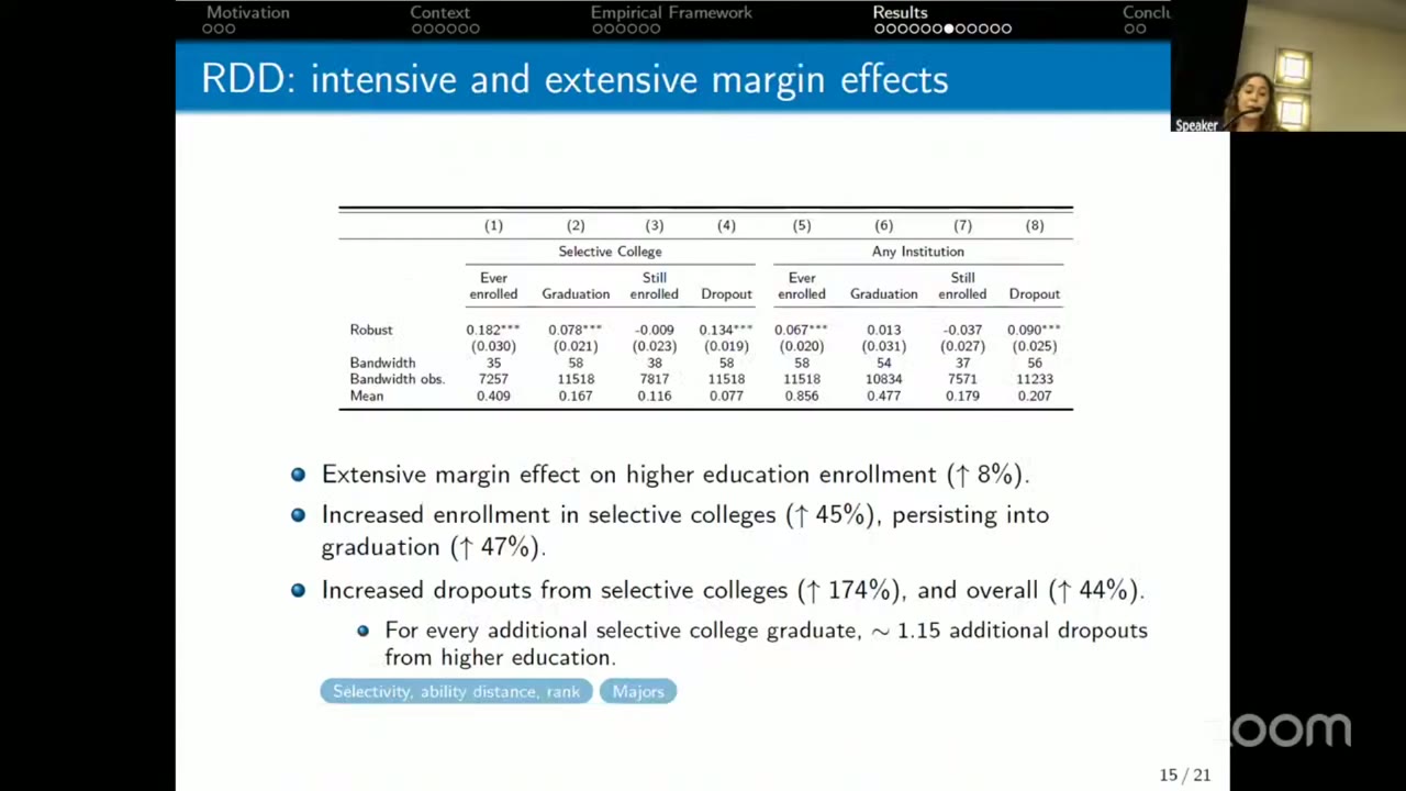
Now go to the students right at the cutoff, who are the weakest the policy reaches. The offer raises selective enrollment by 18.2 points (45%) and selective graduation by 7.8 points (47%). It also raises dropout from any institution by 9.0 points on a base of 20.7% (43% in the paper, 44% on the slide). There is now an extensive margin too (+6.7 points enrolled anywhere). Divide 9.0 by 7.8 and you get Carlana’s summary: “one for one selective college degree more we actually have 1.15 higher education dropout more.” (The paper rounds it to “about 1.2”.) At the margin the option is no longer free.

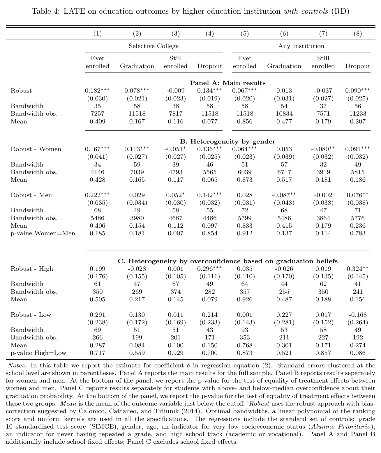
The gender pattern carries over. Marginal women gain 11.3 points of selective graduation, and their share still enrolled at year 7 falls 8.0 points, so their outcomes are settled sooner. Marginal men gain 2.9 points of selective graduation (not significant) and lose 8.7 points of graduation from any institution, with no offsetting rise in still-enrolled. The paper reads that as lost degrees, not delay. Most of the individual gender differences in Panel B are not significant, though (selective graduation p = 0.181). There is still no average labor-market effect at the margin. In the talk’s words, the long-run effect is “statistically significant” and positive for women and “marginally significant” and negative for men.

Who overvalues the option

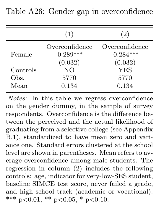
Now the friction the theorem requires. In 2017 the team surveyed grade-12 students in the rct schools (5,770 usable answers) and asked how likely they were to complete a selective-college degree if admitted. They compared the answers with Lasso-probit predictions of the students’ actual chances. Every bin of Figure 7 lies above the 45-degree line. The most common answer was certainty, and the paper reports that fewer than half of the surveyed students who enrolled in a selective college had graduated within seven years, even among those who had said they were certain (p. 31). Men are more overconfident. The female coefficient is −0.289 sd, or −0.284 sd with controls that include the baseline test score. Carlana said “around 0.36 standard deviation”, which is what her slide showed, but the paper’s table and text (“about 0.3”) are lower.

Panel C of Table 4 splits the rdd by overconfidence. For students above the median, the offer raises dropout from any institution by 32.4 points (se 14.5) and selective dropout by 29.6. For students below the median the dropout estimate is −16.8 (se 26.4). The difference has p = 0.086, and the cells have 241 and 192 observations inside the bandwidth, so the paper calls it suggestive. That is a fair description. Overconfident students also end up in programs where their classmates’ baseline scores are further above their own. The pattern is the one the theory predicts: the students hurt by the option are the ones who value it most wrongly. The paper suggests the overconfidence gap “may be a key driver” of the gender split, and “may” is the right verb.

How far

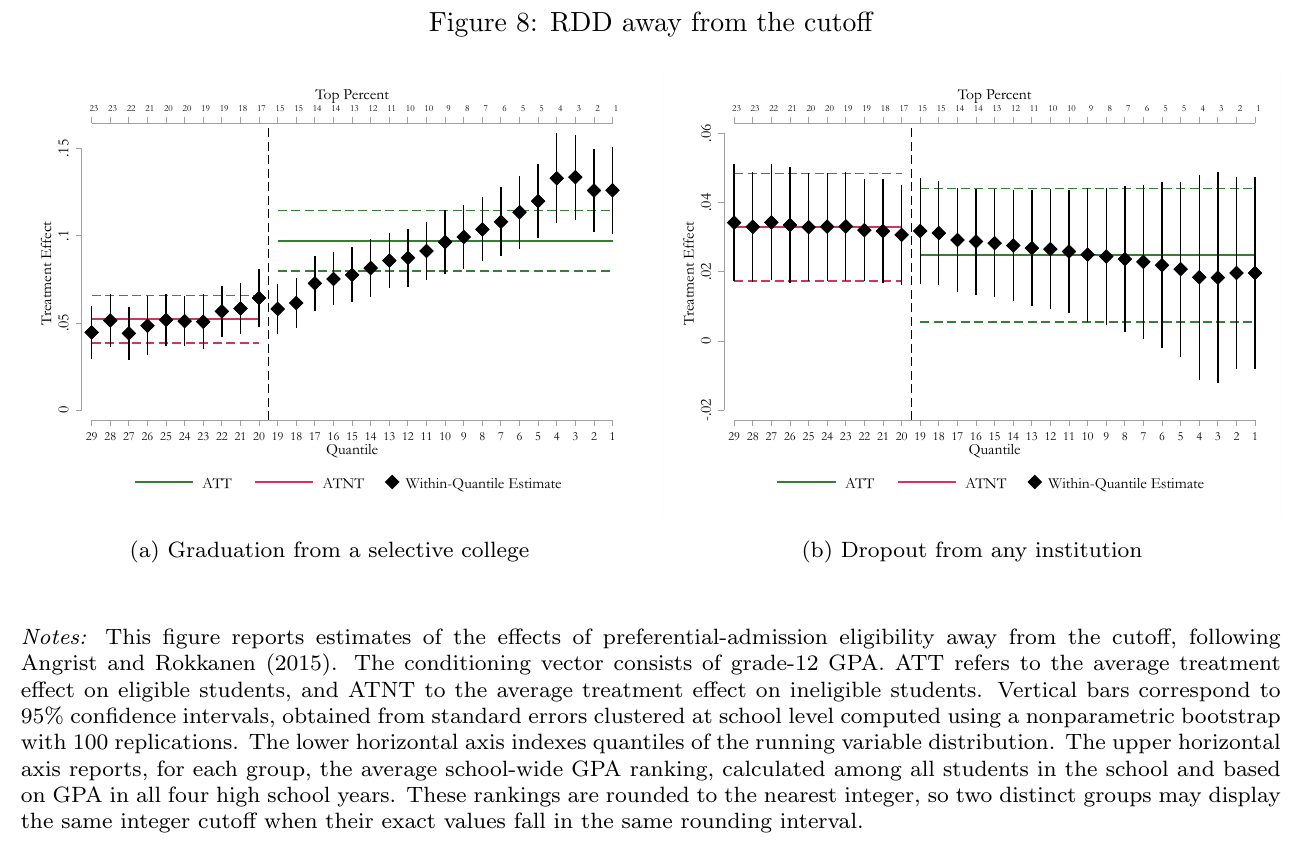
An rdd tells you about the cutoff, and the title asks about everywhere else. To get there the authors use Angrist and Rokkanen (2015): if potential outcomes do not depend on the running variable once you condition on covariates (here grade-12 gpa) and school, you can estimate eligibility effects away from the cutoff. In panel (a), the selective-graduation gains stay positive everywhere, below the current cutoff too, and grow with rank. In panel (b), the dropout effect is positive at every rank, including well inside the group pace already covers. The paper’s finding is that “the first statistically detectable increase in dropout” appears once eligibility goes past roughly the top 6% of each school. In national terms that is about the 60th percentile of grade-10 scores; Carlana said the 58th. Equivalently, preferential admission “could likely be extended to roughly the top 40% of students in terms of high school test scores without generating mismatch-related dropout.” The authors call this an approximate benchmark, not a rule.

The surprising part is where the line falls. pace’s actual cutoff is the top 15%, so the tradeoff already starts inside the eligible group, and the average-only rct never showed it. The word “detectable” also matters. By eye, the dropout point estimates in panel (b) are about the same in every bin. What changes as you move down the ranks is that the graduation benefit shrinks and the confidence intervals narrow. The top-6% line marks where the standard errors become small enough to rule out zero, not where the risk starts. One more thing a careful reader will notice: near the cutoff the extrapolated dropout effects are about 3 points, well below the 9-point late at the cutoff even after scaling by the 85% first stage. The extrapolation uses a different conditioning set, and the paper does not compare the two numbers directly.

The paper also connects its two designs, though the talk skipped this. Theorem 2 gives equation (10), p. 40:

Here $Y_{sa}$ is the potential outcome with pace-school status $s$ and eligibility $a$, $Y_{1*}$ is the outcome in a pace school at whatever eligibility the student actually has, $\pi$ is the share eligible, and $ATT_A$ is the extrapolated eligibility effect on the eligible. The authors find that the rct’s education effects are largely accounted for by the eligibility term. If pace schools do nothing without the reserved seat, the experiment then becomes a LaLonde-style check on the extrapolation, which is a neat use of having both designs in one setting.

The question

There was time for one question, in one minute, from someone not named on the tape. It was the obvious one. Maybe men are just worse at everything; how much of the gender gap is lower test scores, or things the data don’t measure? Carlana said they control for test scores, though the relationship “could be a little bit nonlinear”. She said both sexes are present even among marginal students, with somewhat more women at the very top, and that this is “not enough to justify” the gap: “it seems to be something beyond that.” She could also have cited Table A26, where the overconfidence gap barely moves when the baseline test score is controlled for. That answers the “worse at everything” version of the question better than composition does, though it says nothing about traits the survey never measured.

The limit in the title is drawn in gpa ranks, because that is all an admissions rule can see. What seems to do the damage, suggestively and on small samples, is a belief, and the rule can’t see that.

References