Building Labor Market Statistics with Administrative Labor Market Data

The Federal Reserve Board spent about a decade building a payroll employment statistic out of one private payroll processor’s microdata, and the September 2026 conference draft Ryan Decker presented — commissioned for this conference, so read it as a first public airing rather than a settled paper — is the lessons-learned document. It is unusually honest about something people in this line of work tend to be coy about, which is that the payoff was never a better number. The payoff was a second number.

That distinction is the whole paper, so it is worth being precise about why. The Current Employment Statistics survey is a stratified probability sample of roughly 120,000 businesses and government agencies, about 630,000 establishments, which is something like a quarter of nonfarm payroll employees. Response rates have drifted down to around 40 percent, so the non-response assumptions carry more weight every year. The 90-percent confidence interval on the monthly change is ±122,000. And a business survey structurally cannot see establishments being born or dying, so ces bolts on the Net Birth-Death model, which in many recent years has accounted for half or more of reported payroll gains. Decker’s version on stage: ces “observes truth once a year” [00:27:34], in March, when it is benchmarked to the qcew — a near-census of unemployment insurance tax records covering about 95 percent of jobs, arriving with a five-to-six-month lag. Every other month is benchmarked to nothing. The annual revision gets wedged back across the year, and the monthly wiggles that survive are, in his words, “basically the third print estimate” [00:34:48].

So you would like a second opinion, and adp is an obvious place to get one: roughly 26 million U.S. workers as of June 2025, one in six workers and one in five private-sector workers, about 20 percent of private employment, which Decker noted is “comparable to the size of the ces sample” [00:29:03]. Weekly since July 2009, arriving “with only about a week’s delay” [00:29:13]. Two employment concepts sitting right there in the database — active, meaning anyone on the payroll system, and paid, meaning anyone who got a check.

And then the catch, which Decker states without flinching: these data are not a sample of anything. “Certain types of businesses choose to use a payroll provider. They choose to use a particular payroll provider, and you can’t really observe why they do that” [00:28:16]–[00:28:21]. You never see population truth. The unit isn’t even an establishment; it is a Payroll Account Control, which may be an establishment, a firm, or part of a firm, and the team treated them as establishments because what else are you going to do.

The pipeline, and the wedge inside it

What sits between the raw pay events and a job count is not an estimator. It is a chain of judgement calls, and Decker’s framing of them is the most useful thing in the talk: “you face lots and lots of methodological choices, and you have to make choices, and it’s not always obvious what the right answer is” [00:30:29]–[00:30:34]. Employment gets snapped to Saturdays by a stepwise rule, so a reported headcount applies backward to the whole interval since the last pay event, on the theory that hr departments do not adjust continuously. Weekly growth outside a Davis-Haltiwanger-Schuh band of ±1.8 gets dropped, which is roughly a 100-worker establishment shedding 95 people in one pay period. Surviving units get qcew cell weights on two-digit naics crossed with six size bins, and deliberately not on geography, because state cells multiply the cell count and one large swing in a thin cell whipsaws the aggregate. Ten to twenty percent of accounts have no usable industry code, and the authors assume industry is missing at random conditional on establishment size, an assumption they themselves call “not generally ideal” given that the unassigned units tend to be smaller, younger and faster-growing. Then chain, then seasonally adjust weekly — genuinely harder than monthly, because the n-th Saturday of a month slides by up to a week across years, so the series is not exactly periodic — using the Cleveland-Scott method with explicit holiday effects, on fixed annual factors until 2022 and concurrent thereafter, because the 2020–21 swings had wrecked the fixed ones.

If you want one number for how much of this is discretion rather than measurement: the April 2024 estimate of active employment is −41,000 on fixed seasonals and +59,000 on concurrent. Same data, same team, opposite month. In fairness to everyone, this is not an alt-data pathology. Seasonal-factor revisions account on average for 54 percent of the total revision to the monthly level of ces payrolls.

Then the index is set equal to ces March levels — ces rather than qcew directly, so the team wouldn’t have to handle qcew scope corrections themselves — and the correction wedged linearly back to the prior March. Which leaves the interesting year, the one running forward from the last benchmark, where nothing anchors anything. ces fills that hole with the birth-death model. The Fed team — “it would be a lot of work for us, and we’re a small team” [00:32:57] — did something simpler and stranger: they regressed past adp-frb benchmark revisions on their own lags and added the fitted value as a constant weekly correction to every post-benchmark observation. They call it a forward benchmark and describe it, accurately, as “a very crude analogy to the ces birth-death model,” closer to the bias adjustment ces used before that model existed and that the Census Bureau’s Monthly Retail Trade Survey still uses.

Say plainly what that is. They gave up on measuring business entry and exit and started forecasting their own error instead — and not only the birth-death part of it, but, in the paper’s words, “any other persistent source of measurement error,” selection into adp very much included. It is the kind of move that sounds like giving up until you see the number: between 2005 and 2020 it cut the root-mean-squared benchmark miss from 625,000 jobs to 427,000. Which means the combined unmeasured birth-death and selection bias is, as the authors put it, “reasonably stable and at least to a certain extent predictable over time.” That is a real finding, and a slightly unnerving one, since the thing being forecast is the part of the statistic nobody can see.

Two wrong numbers, wrong in different ways

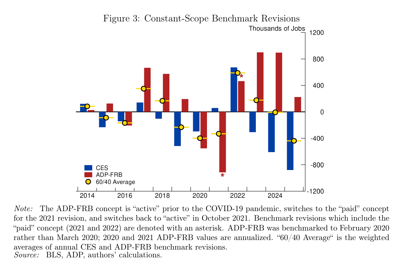
Here is where the paper stops being a methods recital. adp-frb uses no ces input at any stage except the annual level benchmark, so its errors are semi-independent of the survey’s, and two semi-independent noisy signals of the same thing can be pooled. Cajner et al. (2022) did this properly with a state-space model in which true employment growth is ar(1) and each series is truth plus possibly correlated noise; in practice the authors found the fitted Kalman filter is “well-approximated by a simple 60/40 weighted average” — 60 percent ces, 40 percent adp-frb. Those weights are the most recent values of something that moves from sample to sample, not a constant of nature, and the figure deliberately doesn’t print them.

The comparison that makes this work is not flattering to adp-frb on its own terms, which is exactly the point. Its benchmark revisions “are often larger than ces” — the March 2025 value revised up by about 200,000 — but “generally not much larger” and “importantly, are often in the opposite direction,” with ces tending to revise down since the pandemic and adp-frb up. So the blended revision is frequently close to zero and much smaller than ces’s. The useful property of your second estimator is not that it is right. It is that it is wrong differently. And because the blend needs no benchmark to compute, you have it in April, four months before the August preliminary ces benchmark announcement and long before the final one.

Decker gave the room two episodes where this paid: summer 2021, when ces first prints looked like the recovery was “running out of steam” and adp-frb was hotter, and ces later revised up toward it; and 2024–25, when ces was “running really hot,” adp was cooler, and “ces revised down towards us” [00:37:33]. He also, to his credit, did not leave it there, but we’ll come back to that.

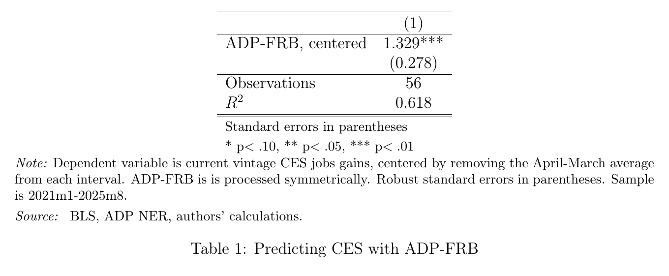
At monthly frequency the relationship survives the obvious objection. Subtract from each series its average April-to-March gain, so both cumulate to zero over every March-to-March interval and the annual-frequency signal — the part the benchmark already guarantees they share — is gone. Regress centered ces on centered adp-frb and you get a coefficient of 1.329 with a robust standard error of 0.278, N = 56, R² = 0.618, over 2021m1–2025m8. The authors flag their own caveat before anyone else can: both series are seasonally adjusted, and correlating the unadjusted versions would give “a false sense of reliability” when the alternative series merely inherits official seasonality.

The month the survey was stale on arrival

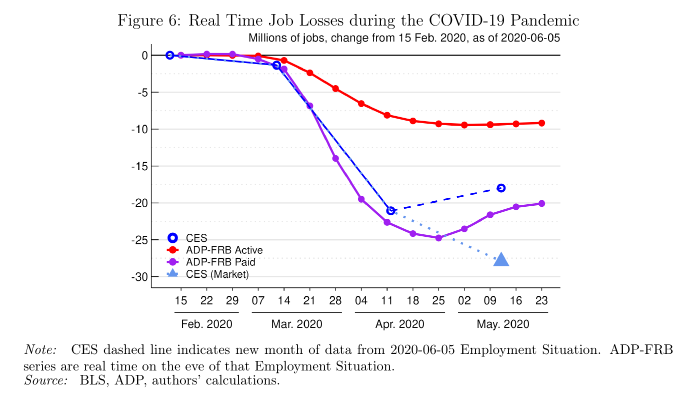
The high-frequency case is the showpiece, and it is genuinely impressive. The team switched from active to paid employment early in 2020 — active keeps furloughed workers on the books, and temporary layoffs went from about 14 percent of job losses to nearly 80 percent — and the paid measure saw things the survey structurally could not. When the 3 April ces print showed about −700,000, later revised to about −1.4 million, adp-frb paid already showed a cumulative decline around 3.5 million, most of it after the March reference period. The paper’s phrase for this is that the ces data “were stale upon release,” which is not a dig at bls; it is arithmetic about reference weeks. By early May the paid series showed cumulative declines on the order of 25 million, very close to what ces would report. And the good one: heading into the June report, the consensus, leaning on claims and other private feeds, expected “several million more job losses” in May [00:39:20], while paid employment in the payroll data had already flattened after the April reference week. “And indeed that is what happened in the ces” [00:39:34].

The wage work gets one slide and deserves more. Because the data are employer-employee level, you can compute each worker’s 12-month wage growth and take a median, Atlanta Fed style, which means composition washes out — roughly 13 million individual monthly wage changes against the Wage Growth Tracker’s 2,000 or so, enough that no three-month moving average is needed. The proof is the pandemic onset, when low-wage job losses drove average hourly earnings growth to an all-time high while the adp-frb medians weakened slightly. One of those is a wage series and the other is a composition series wearing a wage series as a disguise.

The discussant does not let the benchmark off the hook

John Haltiwanger declined to resummarise — “these are outstanding papers,” “the expertise underlying these papers is just enormous” [00:42:40]–[00:42:54] — and went straight to the load-bearing assumption, which is the one the paper is least able to relax. “You can’t get there from here without really high quality benchmark data” [00:43:44], and the adp work “relied very heavily, literally on every step of the way” [00:44:06]. So his first ask is not of the Fed but of bls: quarterly benchmarking from qcew, which market participants already do informally to predict the annual benchmark and which bea already uses in the national accounts. The stated obstacle is known quality differences across quarters, with Q1 the best, and he reads that as a resource problem rather than a methodological one — which in a resource-constrained environment is not exactly good news, but is a different kind of problem.

On the missing industry codes he is blunt: the missing-at-random-within-cells assumption “was a really strong assumption… And we don’t think that’s probably true at all” [00:47:00]–[00:47:04]. Entry into adp is not business entry, but the paper itself hints that client turnover is entangled with genuine entry and exit, “and that’s a source of non-randomness.” His fix is the one everyone keeps arriving at: integrate the payroll microdata with the micro qcew.

On births and deaths he closes the door the forward benchmark was propping open. “The payroll data doesn’t help you really at all on this. Okay, you’re not getting any help here” [00:48:16]–[00:48:18]. Recall that half or more of recent ces payroll gains come from the birth-death model rather than from anyone answering a survey; this is the part of the statistic under the most strain, and the private data have nothing to say about it. His suggestions come from elsewhere — the Business Formation Statistics, which process new business applications weekly in near real time, and ui claims, which are already sitting there.

Where he thinks adp genuinely wins is non-response, and the argument is empirical rather than hopeful. Work with Steve Davis, Jason Faberman and Ian Rucker matching jolts microdata to the bls Longitudinal Database found it is not only closing businesses that stop filing: “businesses that are contracting rapidly aren’t filing reports” [00:50:33]. Which means survey non-response is correlated with the thing the survey measures, in the direction that matters most at turning points. Payroll data mostly sidestep this, because “maybe you don’t respond to the bls survey, but you’re still making your payroll” [00:51:06]–[00:51:08]. A co-author agreed and named the version of the problem that replaces it: once you are in the adp universe you are in, so there is no non-response — what they watched instead was attrition, whether clients leave and whether the leaving is patterned.

A questioner addressed as “John” asked the right follow-up about the two flattering episodes: were there years when adp-frb pulled the wrong way? Decker answered it straight, which is worth noting because he did not have to. There were years when the adp-frb revision was bigger than ces’s and in the same direction, “so if you had taken too much signal in that year it would have erred,” and while it did well in the recent big-revision years, “there were other times in 2017, 2018… when it wasn’t so good” [01:03:20]–[01:03:34]. His co-author added the line that should be printed on the inside of every alternative-data deck: “we don’t want to cherry pick particular cases too much” [01:02:29].

The question that was answered beside the point

The talk was in the past tense from the first minute. Ten years of working with the data; we received new data weekly; we had anonymized microdata access; these private payroll processor data were really useful. Nobody on stage explained why, and the chair had to open the floor before anyone said it out loud.

He opened it to David Wilcox, who prefaced with a line about his wife reminding him to ask the basic questions and state the obvious things, and then stated it: “It feels to me like an obvious thing that hasn’t been stated is it was implicit in Ryan’s comments. Your discussion was in the past tense. adp is no longer providing those data to the Federal Reserve Board” [cap 00:54:32–00:54:43]. That sentence exists only in the auto-captions — the Whisper pass has a gap from [00:54:09] to [00:54:53] and simply does not have it — so it is worth flagging as single-source even though the captions are unambiguous. He went on: “The Federal Reserve Board effort was a live ammunition exercise. We were putting this information in front of the open market committee [cap] and allowing them to make policy decisions because we decided that the product, the blended product, was high enough quality to warrant that — and suddenly it was cut off. What happens if…?” Here the two transcripts do overlap, and they agree verbatim from “the blended product” through “suddenly it was cut off.” They do not agree on “open market committee,” which is the captions’ reading; Whisper hears “community.” Whisper also renders “live ammunition exercise” as “online and in the National Infection Service,” which is its own argument for reading machine transcripts in pairs.

Decker took the question — “this point about the hold-up problem” [01:03:49] — and answered the general mechanism. The Fed’s industrial production statistic has run for over a hundred years as a blended product fed by many private sources, and “over many years we have lost many, many sources” [01:04:10]. The cost of losing one depends on how important it is: “if you were using something like adp, which is so huge, and if you were very dependent on it, it would be very costly to lose it” [01:04:21]. It also depends “on how good your benchmarks are, how soon can you catch it, and can you replace it” [01:04:29]. A very tough problem, he said, but a surmountable one [01:04:42]–[01:04:49 cap].

That is a good answer to a question nobody asked. Note the conditional: if you were using something like adp, if you were very dependent on it. Decker never confirmed the cut-off and never denied it, and neither did any of his co-authors during the rest of the session. The paper says nothing about it either; its abstract is present tense and offers a blueprint, but every empirical verb in it points backward, the wage series stops in July 2025 and the regression sample ends in 2025m8. Read in that light, the paper’s long final section — trusted third parties receiving cell-level growth rates and market shares, secure multi-party computation, secure enclaves, the Boston Women’s Workforce Council wage-gap study, Eurostat’s multi-node enclave prototype, the Danish sugar-beet auction, and a genuinely interesting proposal to have a coding agent run inside the provider’s environment on an outside analyst’s prompt, hedged with the observation that current agents “make amateurish mistakes and are not widely tested on these types of tasks” — stops reading as futurism. It reads as a design for a pipeline that would not be hostage to one vendor’s renewal decision, written by people who have just learned what that costs.

The chair, invoking organisers’ privilege, said the quiet thing in institutional language: ad hoc alternative-data feeds “are basically dependent on contractual relationships” [00:59:50], and an arrangement where payroll data flowed into the official process by design — some to the states for benefits processing, some to bls for statistical processing, coordinated — “is a different infrastructure than ad hoc relationships of purchasing or cajoling data providers” [01:00:24]–[01:00:29]. Michael Stepner of Toronto, whose surname both transcripts mangle, had already made the same point from the other end: the uk reformed its payroll reporting requirements so companies report to government more often, so “rather than making do with the best we can of the qcew to benchmark all these private sector data, what about improving the qcew?” [00:56:38]–[00:56:49].

Haltiwanger’s verdict on the method was delivered before any of that, and it holds up after it. The paper gives a preliminary answer to whether payroll provider data can carry the high-frequency load while benchmark surveys carry the truth, and the answer is: “We’re not ready yet. That’s not a criticism at all. As Ryan said, this is a great supplement to the official data at this point. It’s not a substitute” [00:51:59]–[00:52:14]. What he wants instead is a large-scale demonstration project across multiple payroll providers, in collaboration with bls, integrated with the micro qcew — “the gold standard we ought to be pushing for” — with the access and governance questions split off and parked so the technical question can be tested on its own.

Which is the right sequencing, and also the part the room had just watched fail in the other order. The Fed team solved the technical problem well enough to put the blended number in front of policymakers for years. The access question is the one that ended it, and the paper’s closing lesson — that the usefulness of private administrative data is “conditional on, and enhanced by” high-quality public benchmarks — cuts in a direction its authors state politely and a floor full of people heard plainly. The private signal was never going to replace the public one. It turns out it couldn’t outlast it either.