History Dependence in the Housing Market

Philippe Bracke (Financial Conduct Authority) and Silvana Tenreyro (LSE), “History Dependence in the Housing Market,” American Economic Journal: Macroeconomics 13(2), April 2021, pages 420–443. There is no discussant and no seminar recording behind this piece — it is a digest of the paper itself, not of a talk, so nobody in the room got to push back. The one place the authors speak in their own voice is a three-minute-forty-one-second clip Bracke recorded for CEPR/VideoVox in July 2017, which is quoted at the end and which turns out to be its own small story. Read here: the published April 2021 version plus the April 2020 online appendix.

The house does not know

You own a house. Someone would like to buy it. What is it worth?

The frictionless answer, the one every undergraduate learns, is that the house is worth the present value of the housing services it will throw off — the rent you would otherwise pay to live somewhere like it, discounted, forever, adjusted for the neighborhood and the school and the leaky roof. What you paid for it in 2007 does not enter this calculation. It cannot. The house is a claim on the future, and the price you got it for is a fact about the past that has already happened to you and has no further business being anywhere near the transaction. It is, in the technical term of art that says everything, sunk. Whether the house sells this year should likewise depend on the fundamentals — on whether the current owner’s job moved, on whether a buyer values the property more than the seller does — and not at all on which year the seller happened to sign the last contract.

That is the null hypothesis. Bracke and Tenreyro go and find two identical houses on the same street, being sold in the same year, whose only difference is when their current owners bought, and they check.

Here is the finding, from the first page of the paper: consider two identical houses in the same location, both selling in 2014, one bought in 2007 at the top of the aggregate cycle and one bought in 2001. The 2007 house sells for about 5 percent more, and has roughly 50 percent less chance of selling at all in a given year. (In a footnote the authors add the relevant gap: the 2007 owner is sitting on an expected 2 percent nominal loss; the 2001 owner on an expected 89 percent gain.) The two houses are the same house. The buyers of the two houses are buying the same future. They are paying different prices for it, and one of them is much harder to buy, because of something that happened to a stranger seven years ago.

What “history dependence” literally means

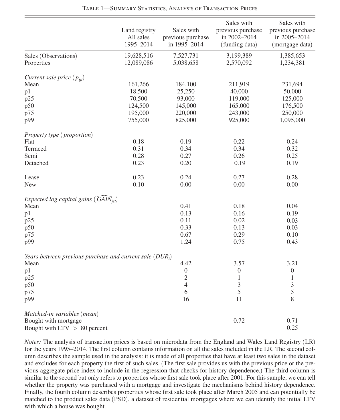
Force the jargon to say what it means. History dependence here is not the owner’s own purchase price mattering — that would be a much weaker and more obvious claim, contaminated by the fact that people who overpay for houses may have bought unusually nice houses. It is the local price index at the date of purchase mattering. The paper’s summary statistic is the expected capital gain, $\widehat{GAIN}_{jst} = \hat\delta_{jt} - \hat\delta_{js}$: the log change in the price index of the owner’s postcode district between the year they bought, $s$, and today, $t$. Expected, not realized. Built entirely out of index differences, deliberately excluding anything specific to the property.

So the variable is, from the individual seller’s point of view, a fact about the calendar. Two neighbors with the same house differ in $\widehat{GAIN}$ only because one signed in 2001 and one in 2007. And what the paper documents is that the market treats those two houses as different goods.

There are two stories for why, and the paper’s real contribution is that it can tell them apart.

The first is credit. This is Jeremy Stein’s 1995 down-payment effect, and it is not a psychological story at all — it is a balance-sheet constraint. Most home sales are to repeat buyers, and most repeat buyers fund the down payment on the next house out of the equity released by selling this one. An owner who bought at the peak has little equity. Selling nets them too little cash to put down on anywhere they want to go. So they set a higher reservation price and they sit tight. Perfectly rational; the constraint is real.

The second is cognitive. Anchoring, in the Tversky–Kahneman sense: in valuing an asset, people overweight an initial cue even when the cue is irrelevant, and the price you paid is a very salient cue. Loss aversion is a special case of this (Genesove and Mayer’s 2001 Boston condominium paper is the ancestor of the whole literature). Slow learning about your own property’s value is another. In all of these, the seller’s reservation price is dragged toward the old purchase price by something that is not on the balance sheet.

The two stories predict identical patterns in the raw data. Both say: bought high, ask more, sell less. You cannot separate them by looking harder at prices.

The design

The data are the pleasure of the thing. HM Land Registry records essentially every residential transaction in England and Wales, and the authors have twenty years of it: 19,628,516 sales on 12,089,086 properties, January 1995 to December 2014, about a million sales a year, with the postcode, the street, the street number and the flat number. Transfers that were not at full market value — divorce settlements and the like — are excluded. Keep only properties that sold at least twice, drop each property’s first sale (it is needed to build the gain), and you have 7,527,731 observations on 5,038,658 properties, mean expected log gain 0.41, mean tenure 4.42 years, mean price £184,100.

The estimating equation is a hedonic regression with a very large amount absorbed:

Equation (3), page 424: $p_{ijt}$ is the log sale price of house $i$ in postcode district $j$ at time $t$; $v_{ij}$ is an individual-property fixed effect; $X_{ijt}$ the time-varying recorded characteristics (new-build, leasehold); $\delta_{jt}$ a year-by-district fixed effect for the current local price level; $\eta_t \otimes \eta_s$ sale-quarter by purchase-quarter dummies for housing seasonality; $\lambda_t \otimes \lambda_s$ every purchase-year by sale-year combination; and $w_{ijt}$ the error. Equation (4), page 425, is the identical specification with a binary “did this property sell this year” indicator $q_{ijt}$ on the left-hand side. The function $f(\cdot)$ is not a slope but sixteen dummies for 0.10-log-point bins of the gain, break-even omitted, so the shape is estimated rather than assumed.

Read that stack of fixed effects slowly, because it is the whole argument. The property fixed effect means the comparison is the same house across its own sales — twenty years of Land Registry lets you follow one address through three transactions, which is why unobserved quality, the standing threat to any gains-based analysis, is simply differenced away. The district-year effect means everyone in the comparison is selling into the same local market at the same moment. And the purchase-year by sale-year interaction absorbs tenure — because prices trended up for most of the period, the gain is nearly a monotone function of how long you have owned, and without this control you would be measuring holding-period effects and calling them anchoring. The identifying variation left over is: differences across postcode districts in the local price path between $s$ and $t$, relative to the national path for that same pair of years, within the same property.

The authors are candid that this control might be doing too much. Footnote 4 on page 424 concedes it “could end up absorbing a substantial amount of variation” in the gain. Hold that thought.

Both margins move, and they move in mirror image

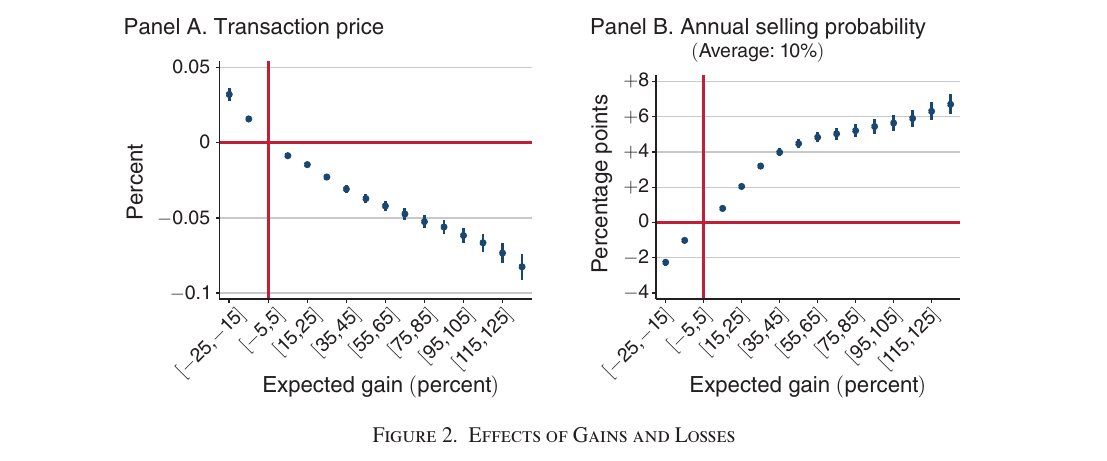
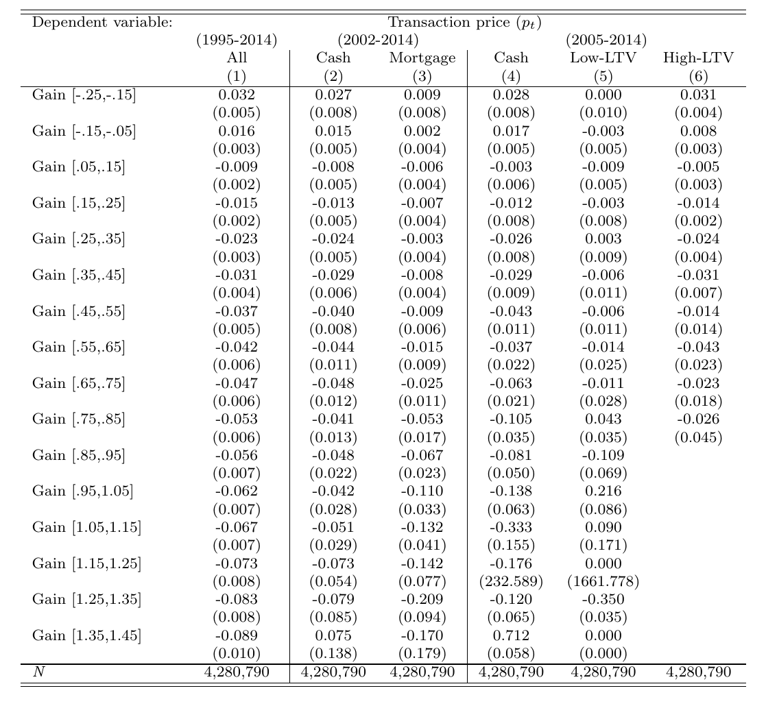
Prices fall monotonically as the expected gain rises. An owner sitting on a 15-to-25 percent expected loss transacts about 3 percent higher; an owner sitting on a large gain transacts lower and lower, out to about 9 percent below break-even at the top of the range. The published text describes the most populated bin — gains of 35 to 45 log points — as “a 4 percent decrease,” which is generous by about a point: the coefficient the online appendix prints for that bin is −0.031.

Selling propensities are the mirror image with the sign flipped: about 2 percentage points less likely to sell at a 15-to-25 percent loss, rising monotonically to about 7 points more likely at the largest gains. The benchmark to hold against those numbers is that the unconditional annual probability of sale among repeat-sale properties is 10 percent. Four extra percentage points on a base rate of ten is not a rounding error; it is the difference between a market and a freeze. And both patterns replicate in all nine England and Wales regions.

The surprising part is that this is mostly not loss aversion

The literature this paper joins is a loss-aversion literature. Genesove and Mayer looked at Boston condominiums in the 1990s, a market where lots of people were underwater, and found that sellers facing nominal losses asked for more and waited longer. The natural expectation is that Bracke and Tenreyro have found the same thing at national scale.

They have not, quite, and the reason is a fact about the sample rather than a subtlety of the estimation. Only about half a million of the 7.5 million repeat-sale observations sit on the loss side at all. The mean expected log gain is 0.41. Almost everybody in England and Wales over these twenty years is up. And the effect is monotone and close to linear over the entire range, which means the mass of the phenomenon lives on the gain side, among winners.

So the actual character of the finding is this: an owner whose local index has doubled since they bought — a log gain of 0.69, so the [0.65,0.75] bin — sells about 4.6 percent cheaper than the identical house next door bought at break-even, and is about 5 percentage points more likely to trade. Sitting on a large paper gain does not make you a tougher negotiator. It makes you a cheerful discounter. The anchor pulls in both directions: it holds losers up and it holds winners down, and because the country is mostly winners, most of the aggregate action is winners quietly leaving money on the table and moving house.

(A caution on units that is easy to lose: the bins are log points, so the eye-catching −0.06 to −0.08 price effects belong to log gains of roughly 0.95 to 1.45, not to a 60-to-80 percent appreciation.)

Switching the credit channel off

Now the trick. Credit frictions require credit. A buyer who paid all cash for the property has no mortgage, no equity constraint of the Stein variety on that purchase, and therefore no down-payment channel to speak of. If history dependence survives among previously all-cash owners, the surviving part cannot be a balance-sheet constraint — it has to be cognitive. The Land Registry records whether a purchase carried a charge (a mortgage) from 2002, so the split is observable.

Equation (5), page 432, where $y_{ijt}$ is either the log price $p_{ijt}$ or the sale indicator $q_{ijt}$; $\gamma_{1k}$ is the bin-$k$ effect for properties previously bought with cash, $\gamma_{2k}$ the additional effect for mortgage-financed ones, and $upto2001$ flags the pre-2002 purchases whose funding is unknown. The braces labelling the two sums “cognitive frictions” and “credit frictions” are printed in the paper; the authors are not being coy about what they think they are measuring. (Equation 6, on the same page, replaces the pre-period indicator with one for pre-2005:I and adds a third braced term, $\gamma_{3k}$, for mortgages whose current estimated loan-to-value ratio exceeds 80 — the median in the regulator’s Product Sales Data and the literature’s usual equity-constraint threshold. Current LTV is imputed by rolling origination LTV forward, amortizing the loan and appreciating the house by the district index.)

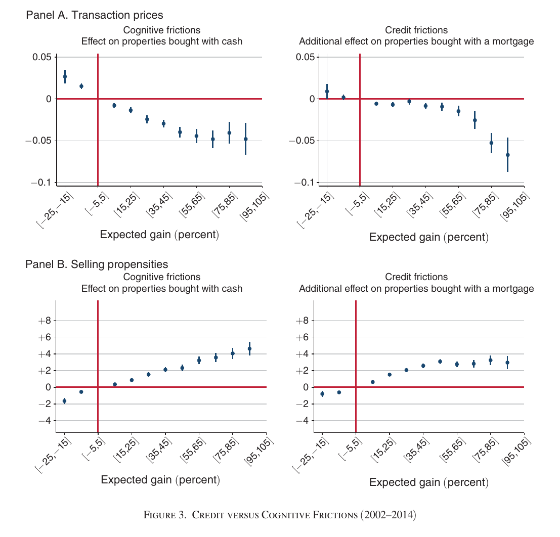
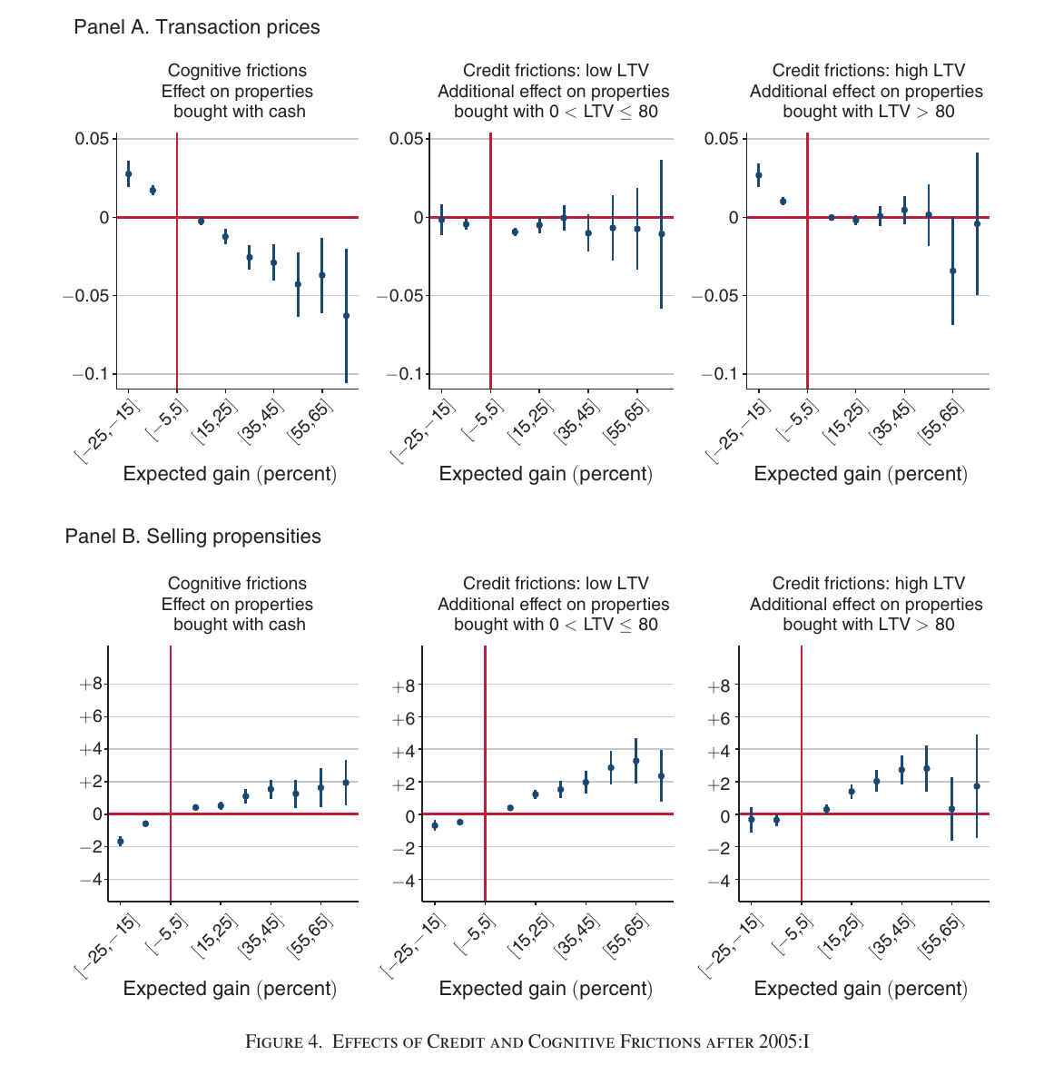
And here is the result, and it is a crossing. Take the benchmark [0.35,0.45] bin. On prices, the cash coefficient is −0.029 and the additional mortgage effect is −0.008: the all-cash owners, who have no down payment to raise, reproduce almost the entire price effect on their own, and leverage adds very little. On selling propensities the ranking reverses: the cash coefficient is +0.021 while the additional mortgage effect is +0.026, stacked on top — and in the post-2005 window there is a further +0.027 for the high-LTV group on top of that. The cash coefficients on the selling side are statistically significant mainly at large gains.

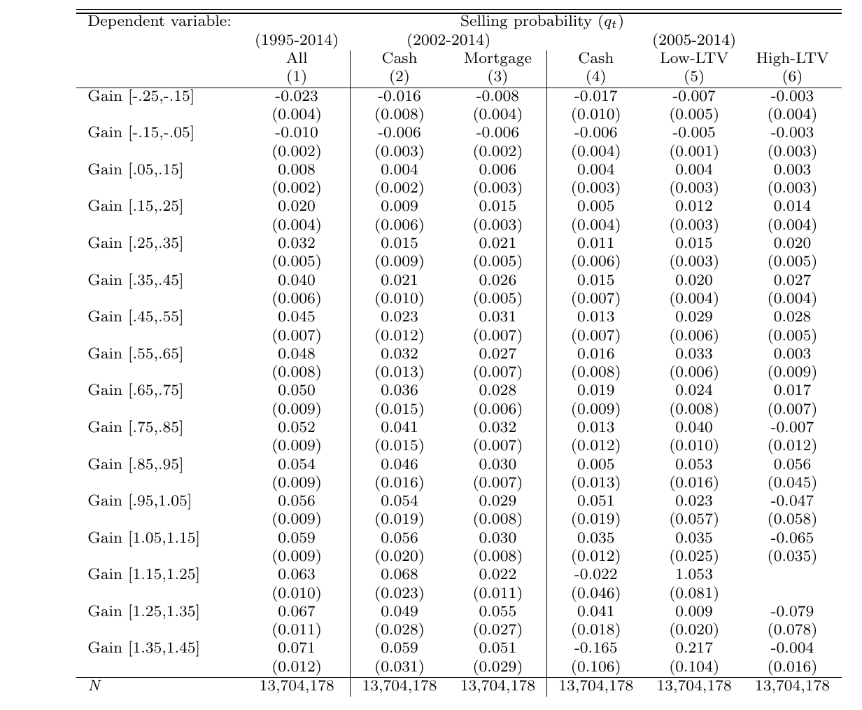
That crossing is the paper’s real contribution, and it is worth stating in plain words: cognitive frictions carry the price effect; credit frictions carry the selling-propensity effect. You do not need debt to make someone hold out for a number anchored to what they paid. You do need debt to stop them moving. The wedge in what you ask is in your head; the wedge in whether you go is on your balance sheet.

Two honest qualifications, both of which the paper carries and neither of which it fully disposes of. Nothing here is randomized: nobody assigned households to pay cash or to lever to 90 percent, and cash buyers are wealthier, older and more investor-heavy than everyone else. So the correct verb is consistent with, not caused by. And the inference is deliberately one-directional — the authors say so on page 421 and again on page 431. Finding history dependence among cash buyers proves cognitive frictions bite. Not finding it would prove nothing, because cash buyers might simply be people for whom anchoring works differently. The design can confirm the cognitive channel; it cannot refute it.

It is also worth noticing that “cognitive frictions explain most” means the cash coefficients are large and significant, not that the credit add-on is nil. In the post-2005 price columns, at the largest loss bin, the additional effect of a high-LTV mortgage is +0.031 on a cash baseline of +0.028 — as large again. And there is a genuine inconsistency in the record here: the published Figure 4 plots the high-LTV price point at [0.35,0.45] slightly above zero, while the April 2020 online appendix table prints −0.031 with a standard error of 0.007. The chart also stops short of the bins the table reports. The cause is unresolved, likely a version difference, and the two are not interchangeable sources.

The kink

Because the effect is estimated over the whole range rather than only on the loss side, the paper can run a second, independent test for reference dependence: does the response kink at zero? Prospect theory says the value function is steeper for losses, so it should.

Equation (7), page 436: the sixteen bin dummies are replaced by one linear gain term with slope $\gamma_0$, plus $\gamma_1$, an extra slope that applies only below the threshold $x$, tried at 0, 0.2, 0.4 and 0.6.

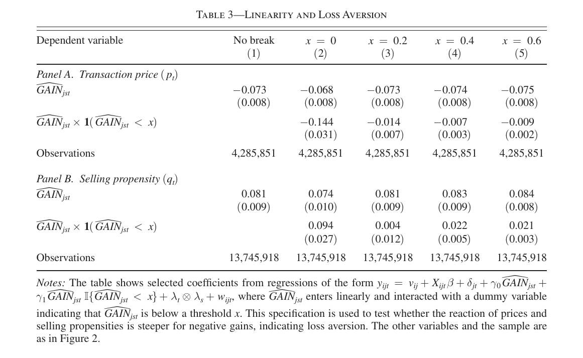
The table does two things at once, and the second is the more interesting. With no break, the linear slope is −0.073 (0.008) for prices and +0.081 (0.009) for selling. Impose a break at zero and prices get an extra loss-side slope of −0.144 (0.031); selling gets +0.094 (0.027). So the kink is real — reference dependence at the nominal zero is in the data, and the break at zero is the largest of the four thresholds tried, significant for both outcomes. (The paper’s prose also calls zero the most statistically significant threshold, which the printed selling panel does not support: the coefficient-to-standard-error ratio there is about 3.5 at $x = 0$ against 4.4 at 0.4 and 7.0 at 0.6. No fit statistic is reported anywhere, so nobody should say zero “fits best.”)

But look at what happens to the linear term when the kink is admitted: −0.073 becomes −0.068. The kink barely eats into it. Most of history dependence is not the kink. It is the long, smooth, boring slope running all the way across the gain distribution, which is exactly the anchoring story rather than the loss-aversion story. And the extra loss-side slope is about 50 percent larger for prices than for selling propensities, which lines up with the cash/mortgage split: the cognitive machinery is doing more work on what you ask than on whether you move.

Does any of this add up to a macro number?

England and Wales transactions peaked in 2007, collapsed, and had not returned to the pre-crisis level seven years later. Meanwhile the price index dipped and resumed climbing. That divergence — prices resilient, volumes flat on the floor — is the puzzle the paper was written to speak to.

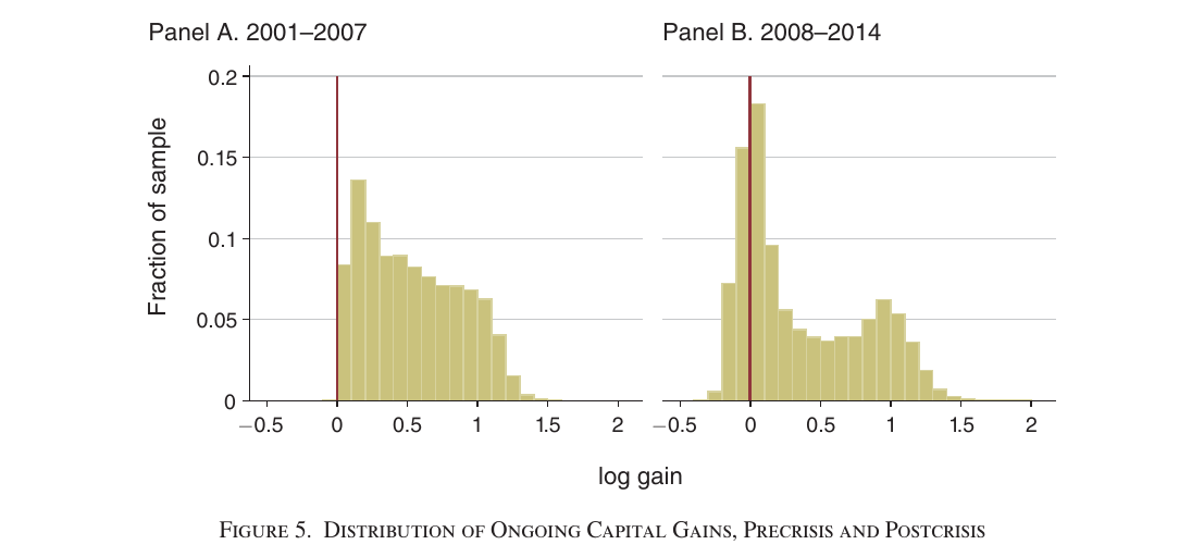
The mechanism, if it works, works through the distribution. In 2001–2007 practically nobody had an expected loss and the mass sat comfortably in the 0-to-100 percent gain range. In 2008–2014 a loss tail appeared and a great pile of properties accumulated right at zero — owners whose local index had gone precisely nowhere since they bought. Push that population through the selling-propensity coefficients and you get fewer transactions, because the coefficients say people near zero do not move.

So the arithmetic, exactly as the paper does it and with the full frame it needs: the average annual selling propensity for a property fell from 7.7 percent in 2001–2007 to 3.3 percent in 2008–2014, a drop of 4.4 percentage points. Multiplying the change in each gain bin’s share by that bin’s selling coefficient from Figure 2, and summing, gives −1.4 percentage points. History dependence accounts for about one-third of the fall. Running the same reweighting on the price coefficients says house prices would have been about 1 percent lower without history dependence. Both numbers use all properties in the 10 percent random sample, not just the ones that sold — the annual-sale panel is built from every property from its first appearance, over 120 million property-years before sampling, so this exercise does not inherit the multiple-sale selection that constrains the price side.

This is a partial-equilibrium reweighting and the authors label it as such: “suggestive of the potential impact of history dependence rather than a precise quantitative estimation of general equilibrium effects.” It is not a bound in either direction; the paper derives none, and neither should anyone reading it. The obvious missing feedback is that a seller who withdraws from the market is also a buyer who withdraws from the market, so whether general equilibrium would raise or lower the one-third is not established, in either direction.

A corroborating look at the listings

The last section matches the Land Registry to WhenFresh’s feed of every daily listing on Zoopla from November 2008, which lets the paper watch the seller behave rather than only observe the outcome. (Caveat the authors flag: Zoopla is agent listings, and about 11 percent of UK homes sold privately in 2010.)

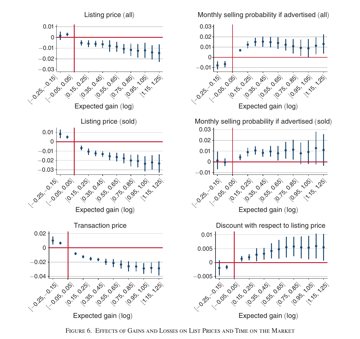
Sellers expecting losses post higher asking prices; sellers expecting gains post lower ones, and get out faster. At the [0.35,0.45] bin the list price is 0.6 percent lower across all listings and 1.3 percent lower among listings that eventually sell; by [1.15,1.25], the largest bin the published chart shows, those are 1.5 and 2.3 percent. The monthly probability of selling once advertised is 1.5 points higher at [0.35,0.45] among all listings but only 0.8 points higher among eventual sales — discounting is what makes the sale happen.

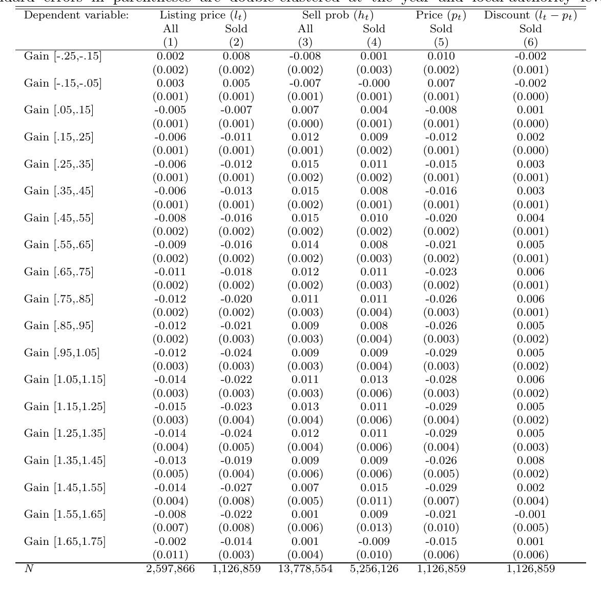
The quiet result in the bottom-right panel is that the implied list-to-transaction discount barely moves — the plotted point estimates peak around half a percentage point at the largest displayed gains, which the published text describes as “reaching around 1 percent for properties with large expected gains.” Transaction prices fall about as much as asking prices do, which is to say sellers have enough bargaining power to pass their history premium straight through into the price the buyer pays. The anchor is not just a fantasy in the listing; it survives negotiation.

One more decomposition, in the appendix, complicates the story usefully. Split the annual selling propensity into deciding to list and selling conditional on being listed, and the listing margin is essentially flat — no significant effect of expected gains on the probability that a property appears on the market at all (average annual listing probability 1.5 percent), except that owners with losses above 15 percent list less. The evidence therefore points toward conversion — whether a listing becomes a sale — as the operative margin. But the paper never quantifies what share of the annual selling effect runs through conversion, and the listing measure is agent listings only, so this is a direction, not a decomposition.

Where it is thin, since nobody was there to say so

The authors run the objections on themselves, which is more than many papers do, and they lose some of them.

The strongest answer they have is on mean reversion, the standard killer of gains-based analyses. If your measure of the gain quietly contained the property’s own pricing error at purchase — as Genesove and Mayer’s does, since theirs subtracts the purchase-date residual — then a house that sold unusually high last time shows a smaller measured gain, and mean reversion would tie the measured gain to today’s price mechanically. Bracke and Tenreyro’s measure is built from index differences only and never touches the residual, so the channel is closed by construction. Appendix C is better still: putting the residual back in alongside property fixed effects flips the price coefficients’ sign, which is a textbook Nickell dynamic-panel artifact rather than a finding, and controlling for the residual explicitly or dropping the fixed effects restores the paper’s pattern.

The weakest is the claim that the kink test is “orthogonal to the distinction between constrained and unconstrained sellers.” It is not, quite. A down-payment constraint binds at a threshold in equity, and for a household that levered to 80 or 90 percent LTV, zero equity headroom sits very close to zero nominal gain. A kink at zero is consistent with prospect theory and with a binding equity constraint, and the comparison of relative kink sizes across the two outcomes (−0.144 for prices against +0.094 for selling) is carrying more inferential weight than the identification can support.

Two more are conceded rather than answered. Unobserved quality is handled by the property fixed effects, but time-varying quality is not: the robustness check drops properties flagged as altered in the Energy Performance Certificate register, which effectively begins in 2008 and records changes to floor area, roof, walls and windows — that is, structural fabric, not kitchens or bathrooms or a coat of paint. A seller sitting on a large gain who skips the pre-sale refurbishment would produce the price result with no anchoring anywhere in it. And selection into sale is acknowledged and never corrected: the price regression conditions on the house having sold, and the paper’s own second result is that the gain determines whether it sells. The diagnostic offered — that discounts on large-gain properties are larger among listings that sold than among all listings — is direct evidence that the selection is real. The sign of the resulting bias in the price panel is never established.

Then there is the tenure control. Drop the purchase-year by sale-year interactions and the price results survive but the selling-propensity magnitudes blow up; replace them with duration dummies and the shape holds while the magnitudes move a great deal (the [0.35,0.45] price effect lands near −0.07 against a baseline of −0.031). The direction is robust. The exact numbers are not, and it is the aggregate exercise — a reweighting of exact coefficients — that cares about exact numbers. Combine that with footnote 4’s concession that the control may be absorbing a substantial share of the variation of interest and the honest summary is that the selling-propensity result is the one most dependent on getting this control right.

Finally, the price sample requires three recorded transactions in twenty years, which selects a high-turnover, flat-heavy slice of the housing stock and excludes new builds structurally. Dropping the property fixed effects preserves the pattern with effects bending toward zero at large gains; replacing them with full-postcode fixed effects gives results “similar to the baseline case but a little smaller quantitatively.” “A little smaller” is doing quiet work, since the headline price magnitudes come from the most selected sample and then feed the price counterfactual. The criticism does not carry over to the volume side, which never required repeat sales in the first place.

What Bracke said in 2017

Which brings us to the clip, and to the small pleasure of watching a paper get refereed.

In July 2017, Bracke recorded three and a half minutes explaining this work. He describes the identification exactly as published — same house, same local area, compare them one against the other and check when they were first purchased. Then he gets to the mechanism, and says this about the cash-versus-mortgage split: “if the mortgage based explanation the one that relies on deposit is the one work we should see no effect in in the cash group however we see the same history dependence and with approximately the same intensity in both groups which leads us to think that the behavioral explanation is the one really at work in the UK housing market.” And then the headline: “about 10 percent of the decline in housing market sales after Great Recession in the UK can be explained with history dependence.”

The published abstract, four years later, reads: “cognitive frictions explain most of the history dependence in sale prices, whereas credit frictions are more relevant for selling propensities.” The 2017 verdict — behavioural, full stop, same intensity in both groups — turns out to be right about prices and wrong about volumes, and volumes are the margin the video’s own motivating question (why did sales collapse?) actually needs. And the aggregate headline went from about 10 percent to about a third. Those are not demonstrably the same calculation — the clip states no baseline years, no horizon, no sample and no method, so what is established is that the stated headline changed, not that one number tripled.

The paper’s closing thought survives both versions intact, and is stated as a conditional trade-off rather than a law: higher house price growth could spur more housing market activity today, but it raises the need to sustain that growth later, “feeding in the unsettling need for potentially spiraling house prices.”

Which is a polite way of saying that a market whose volumes depend on how much its participants think they have made is a market that has to keep making them money to keep functioning. The frictionless model says what you paid is sunk and irrelevant. Nineteen and a half million transactions say the number is still sitting there in the seller’s head, and on the seller’s mortgage statement, quietly setting the price of a house it has nothing to do with.