Credit expansion and credit misallocation

Alexander Bleck (UBC) and Xuewen Liu (HKUST), Journal of Monetary Economics 94 (2018), 27–40. Presented by Bleck at the Federal Reserve Bank of Atlanta’s 22nd Annual Financial Markets Conference, Research Session 1, May 2017; discussant Julia Coronado, MacroPolicy Perspectives. Written from the published version and its online appendix.

The published article is a theory paper that reaches its first equation on page four and never shows you a picture of China. The talk is not like that. Bleck opens at the Atlanta Fed with about seven minutes of charts, none of which survived into print — the article’s empirical section has no figures at all — and those seven minutes are the best available answer to why the paper exists.

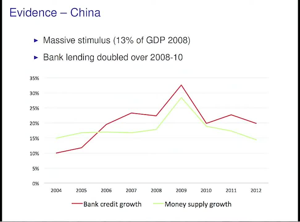
He picks China for two reasons. The package was “about twice that of the United States by some measures, 13% of GDP at the time,” and China is “a very much heavily bank-based system” (00:03:52) — so if you want to know what happens when stimulus has to pass through a banking system on its way to the real economy, this is the clean experiment. On the funding-composition chart the bank-lending block “about doubled in one year.” He is deadpan about the graph itself: “It’s not a very sophisticated graph here.” Then: “I would call that a massive stimulus.”

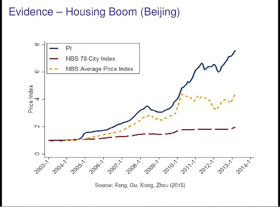
The money went somewhere, and the somewheres are the ones you would guess. Beijing house prices — “this is, of course, cherry-picked a little bit,” he concedes, with an aside that his own Vancouver looks much the same. Shanghai “looks not too different.” Production commodities, stripped of food and fuel, “just about doubled, a lot of which was attributed to China.” And: “I ran out of graphs here, but if you looked at the stock market in China, that pretty much followed a very similar pattern.”

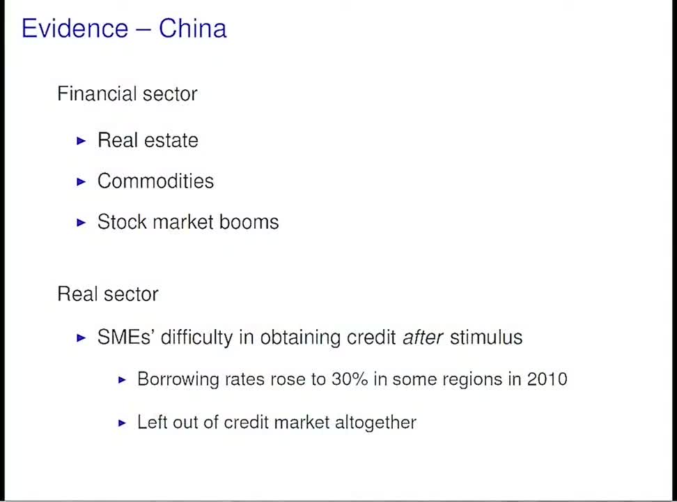
And then the slide that is the entire paper. Small and medium enterprises, “that still make up the chunk of the economy even in China,” did not get cheaper credit. “Things looked actually worse than they looked before the stimulus. That is, there were lots of places where actually their borrowing rates increased after the stimulus, not decreased, which is what you would expect from traditional explanations of monetary policy.” Underground rates reached 30% in some regions. And some firms “were totally left out of the credit market altogether after the stimulus” (00:07:10).

So: you doubled the credit in the system, and the borrowers you were aiming at came out worse. The available explanations are mostly about bad actors — the lending was politically directed, or the banks were captured, or it was a bubble and bubbles are irrational. Bleck and Liu’s claim is that you do not need any of that. Hand the money to a competitive banking system that lends strictly against collateral, with no favouritism, no bubble and no irrationality anywhere, and past a threshold it will take credit away from the sector you were trying to reach. Not less than it might have. Less than before.

The mechanism

Two sectors, identical in every respect but one. The one is asset specificity, written $X$ — the cash flow an outside creditor could recover if it seized the borrower’s capital and operated or resold it itself. Force the jargon to say what it means and it means: how much is this stuff worth to somebody who isn’t you. Bleck’s version in the room is better than the paper’s (00:27:09): you don’t “have to be an expert to know how to live in a house,” whereas “the machinery of a specialized car maker that only can make cars by that car maker… won’t be able to find as many buyers, won’t be able to fetch as high a price.” Commodities and securities, he adds, “by their very name, they’re commoditized.” Sector 1 is the specific-asset sector — manufacturing, mining, transport. Sector 2 is the redeployable one — finance, trade, construction, real estate.

$X$ does two jobs one period apart, and the paper is easy to misread on this. In the secondary market where seized assets get resold, $X$ is the margin a speculative buyer can borrow against each asset he holds — so a higher $X$ means buyers can bid the resale price up. And that resale price is then the ceiling on what a firm in that sector can borrow at date zero, because nobody can commit to repay more than what the lender could liquidate for. That is equation (1), p. 31:

$B^{*}$ is the marginal borrower — an entrepreneur whose external financing need is at most $B^{*}$ gets funded, one whose need exceeds it does not — $P$ is next period’s resale price of the collateral, and $r$ is the real interest rate. This tiny equation is the whole transmission device, and we will come back to it in a minute with a certain amount of violence.

The resale price itself is cash-in-the-market. Whoever is optimistic about the terminal payoff buys; whoever is pessimistic sells; the price is what the optimists’ money can cover. The interior branch of equation (3), p. 31, with the credit-market clearing condition substituted in:

The numerator is the buyers’ own funds — the measure $\pi$ of optimists, holding their project cash flow $C$ net of debt service plus their withdrawn deposits — plus the margin $X$ they can borrow per asset; the denominator $1-\pi$ is the float being sold; $Q$ is the government’s liquidity injection; $f$ and $F$ are the density and distribution of firms’ external financing needs. Note what is not in it: no belief parameter appears in the interior branch at all. Optimism decides who trades and sets the ceiling and floor between which the price must sit; inside those bounds the price is just money divided by float. The paper’s own gloss is that the price reflects “not only the asset’s expected future fundamental value at $T_2$ but also the current liquidity that buyers can access at $T_1$.” (One maintained assumption rides quietly here: the authors select the equilibria in which sellers have enough funds to meet the buyers’ borrowing demand.)

Now run it. Inject liquidity, banks lend more, more firms clear the threshold, more firms means more cash in the hands of secondary-market buyers next period, resale prices rise, collateral values rise, banks lend more still. Standard Kiyotaki–Moore amplification, and within a single sector it is entirely benign — “that you would think is a good thing for everyone in this sector,” as Bleck says.

The trick is that the loop has a gain, and the gain is $X$. When $X$ is low enough, the buyers have so little margin capacity that the price never lifts off the pessimists’ valuation no matter how much you inject; it sits pinned at the floor for every feasible $Q$. Sector 1’s loop is not weak. It is dead. That is Proposition 3, p. 32 — and the paper is careful to call this “the cleanest case” rather than the requirement. Footnote 13 keeps the results when both sectors sit above the cutoff, with both prices moving, provided the stimulus capacity is not too large. What the mechanism needs is asymmetry, not paralysis.

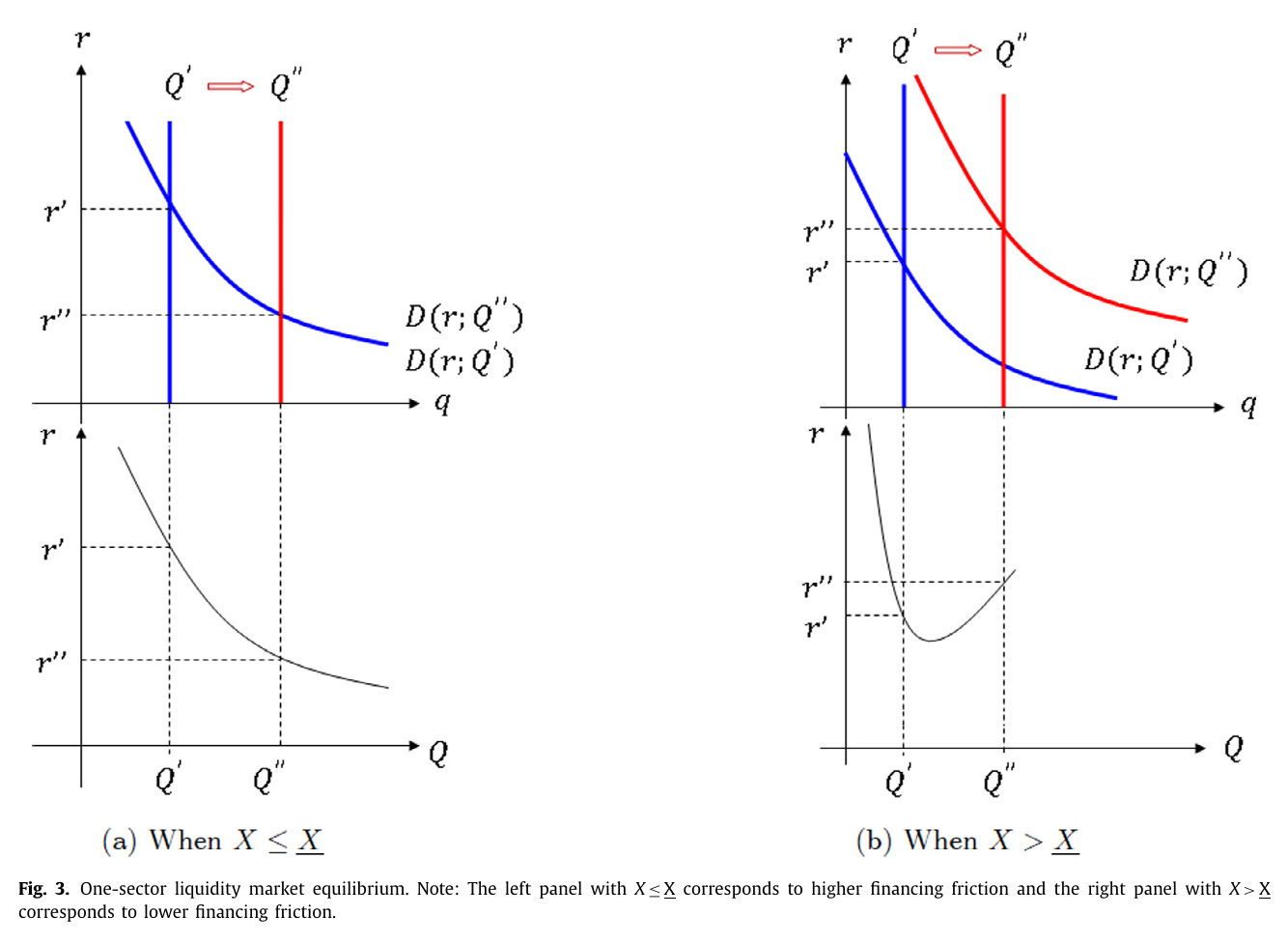
Here is the first thing that should bother you, and it is a one-sector result before any cross-sector story appears. Injecting loanable funds shifts the supply of credit out, which lowers the rate. But it also raises collateral values, which qualifies more borrowers, which shifts the effective demand for credit out too. If the second shift beats the first, the interest rate goes up when you add liquidity. Bleck’s spoken version (00:16:03): “the supply of liquidity affects and causes the liquidity demand to change” — followed immediately, and honestly, by “now most of the time, I’ll say, this actually goes in the right direction.” The online appendix, in the proof of Proposition 4, gives the exact condition:

The rate rises exactly when the density of firms bunched at the margin, $f(B^{*})$, is thick enough that one more entrepreneur crossing the threshold adds more liquidity to next period’s asset market than the injection added to the loan supply. Proposition 4 establishes only that this happens “under some distribution $f$ and some parameter values” — an existence claim, not a generality claim, and it should be read as one.

One price, two sectors

Now put the sectors together, and notice the asymmetry in what is shared. The date-one asset markets are segmented: nobody in mining bids for the resale of a Shanghai apartment. But the date-zero credit market is integrated — one banking system, one real interest rate. That is the only thing connecting the two sectors, and it is where the entire result lives. Equations (5a), (5c) and (5e), p. 34:

One rate $r$, sector-specific prices $P_i$ and thresholds $B_i^{*}$, and an adding-up constraint saying the injection has to end up somewhere. And now go back to equation (1) and read it as a lender in Sector 1. Your borrowers’ collateral is pinned. The rate is not. So $B^{*}_1 = P_1/(1+r)$ falls, mechanically, because the denominator moved and the numerator can’t. Fewer of your firms qualify. You lend less. The funds you don’t lend go into the common pot, which is to say into Sector 2, which raises Sector 2’s collateral values further, which raises the rate further, and so on around again.

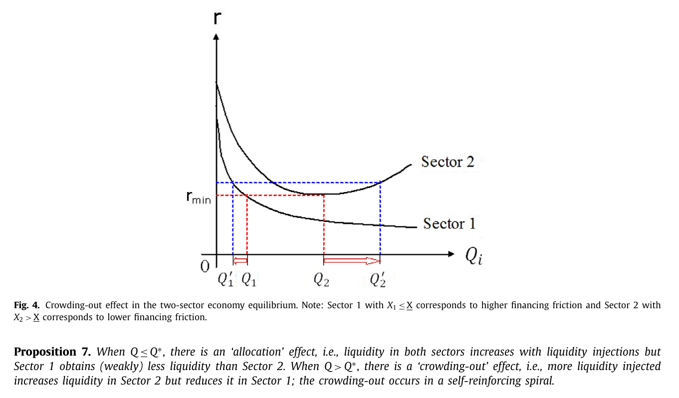
That is Proposition 7, p. 35, and it comes in two regions. Below a threshold injection $Q^{*}$ there is an “allocation” effect: everybody gains, Sector 1 just gains less. Above $Q^{*}$ there is a “crowding-out” effect: more injection raises Sector 2’s liquidity and reduces Sector 1’s, “in a self-reinforcing spiral.” Bleck narrates the spiral with numbers he makes up on the spot, which is the clearest statement of it anywhere (00:24:26): Sector 1 firms “might have received a hundred million dollars before the stimulus; after this excessive stimulus, they may only receive 80 million. The extra 20 go into sector two. And that may then further appreciate, lead to further investments, further appreciate the collateral value, lead to further relaxation of these borrowing constraints, further competition for money, interest rate goes up, and that crowds out more money out of the initial sector.” The object that survives the storytelling is a multiplier: Sector 2’s inflow exceeds the aggregate injection.

Be careful with the word “spiral,” and the paper mostly is. There are three dates and one credit market; nothing runs along a calendar. The spiral is a tâtonnement narrative for why a comparative-static multiplier exceeds one — the standard way of talking a reader through a fixed point — not a dynamic boom-bust. Nobody at the conference challenged this, incidentally, which is either a compliment to the exposition or a warning about it.

He also names the thing the published paper never names (00:25:12): “There is an externality from sector two to sector one: sector two attracting the money hurts sector one.” The word “externality” appears nowhere in the article.

What is actually proved, and what merely can happen

Now the part where a theory digest usually cheats, so let us not.

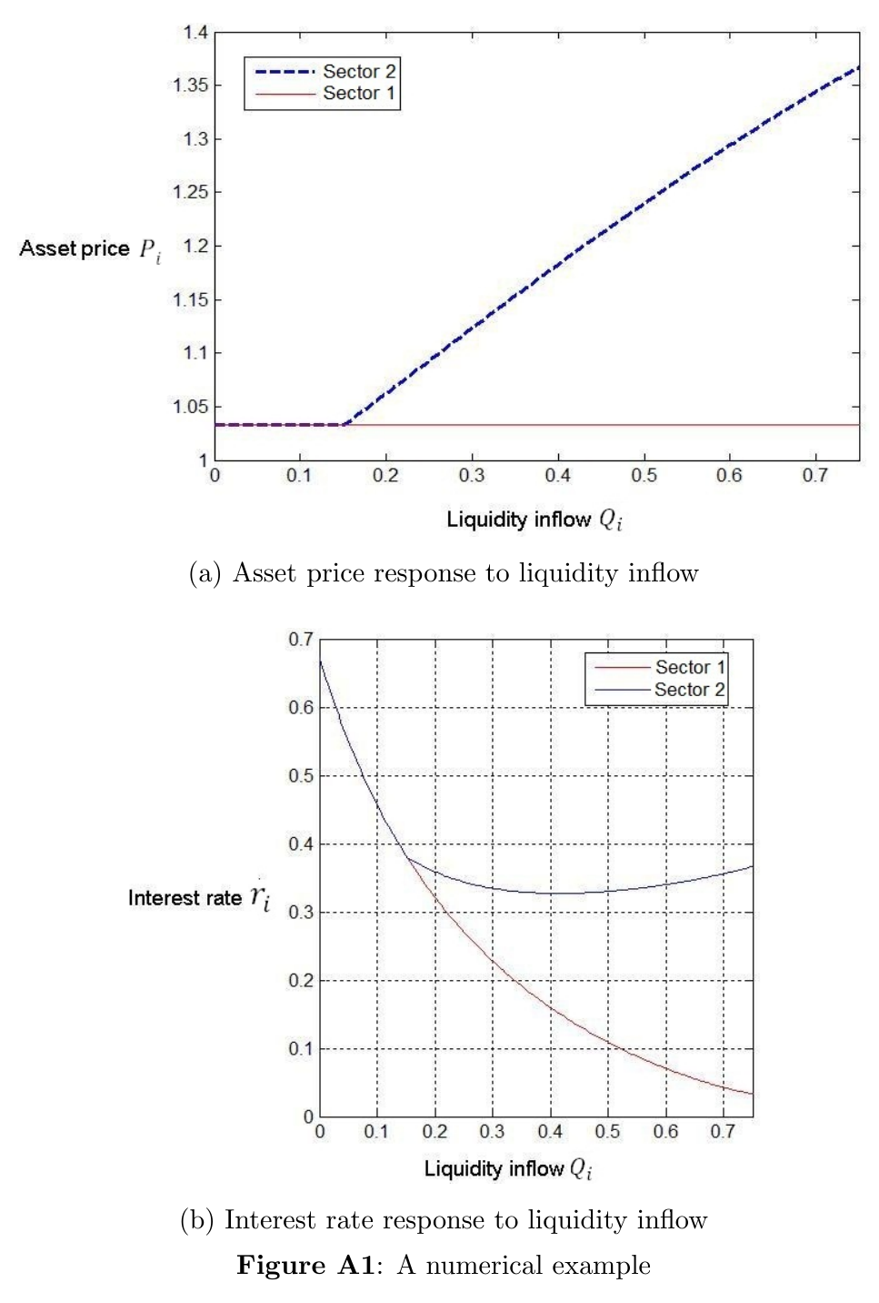
Crowding-out, in the baseline, is not a welfare loss. The two sectors there have identical surplus; Sector 2’s investment is genuinely positive-NPV, not a bubble. And aggregate liquidity investment rises with the injection throughout, crowding-out region included — the composition tilts, but the pie grows. So Proposition 7 is a lopsided expansion, not a transfer and not a misallocation. The appendix’s worked example for Propositions 3 through 7 makes the point sharply, because it gives both sectors one common cash flow: even with returns exactly equal, Sector 2 takes roughly 68% of the injection at the optimum, and its share only grows past it. The uneven split is not a return story. It is a collateral story.

Misallocation requires an extra assumption, made in Section 4.2 and not derived from anything: that the high-friction sector is also the high-return one. That is Proposition 8, p. 36, which needs the belief mass $\pi$ small and the density $f$ thick in some region, and which is illustrated in a second, separate parameterisation with the sector cash flows split 5.6 against 4. Proposition 10, the actual welfare statement, holds under those same conditions and additionally “under some parameter values” — and its optimum is a different object from Proposition 8’s threshold. In the numerical example they land on the same number, and the appendix flags that as “coincidentally,” which is a word worth reading twice. Corollary 9 says aggregate returns to capital fall past the threshold, which sounds like a diagnostic until footnote 24 concedes they can fall below it too.

There is a genuinely elegant thing buried in that corollary, though. The return to capital in each sector is a constant by construction — no diminishing returns anywhere in the technology. Aggregate returns to capital nonetheless decline, entirely through the composition weight shifting toward the lower-return sector. Decreasing returns manufactured out of nothing but arithmetic.

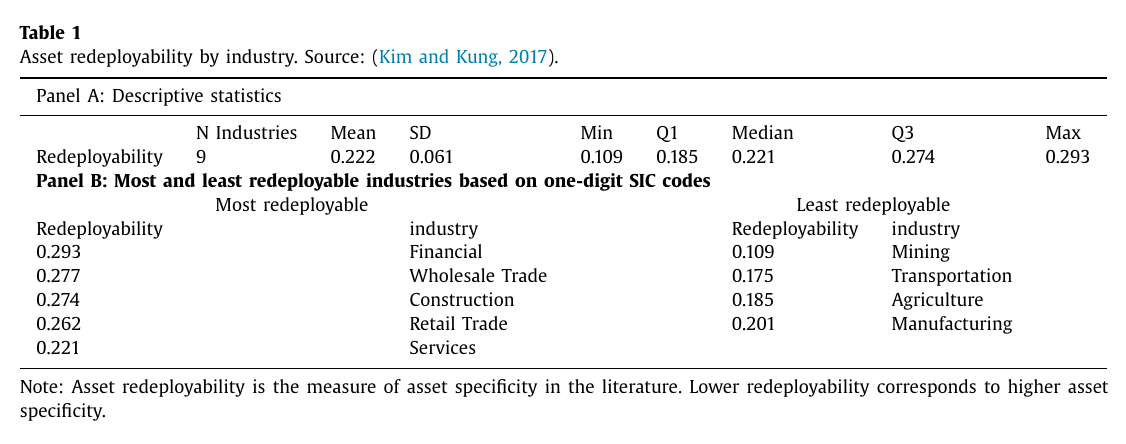
The empirical section is a narrative review of other people’s work plus the motivating episodes — no dataset, no regression, no identification claim. Its one quantitative exhibit is reproduced from Kim and Kung (2017), and it carries exactly what it needs to: the ordering the model assumes is real, with finance, trade and construction at the redeployable end and mining, transport and manufacturing at the specific end. The section also states three falsifiable implications of low specificity — higher recovery rates, more secondary-market trading, higher leverage — and points at published work supporting all three. What it does not do, and does not claim to do, is test the crowding-out channel. Note too that the euro-periphery evidence is mapped by the authors themselves onto the allocation region, the uncontroversial half where both sectors gain and the rate falls.

The surprising thing

The rising interest rate is the narrative spine of the entire paper. Every explanation on pages 28, 34 and 35 runs through it — the higher rate discounts Sector 1’s frozen collateral, so Sector 1 shrinks. Bleck leans on it harder still in the room; asked for a practical tell that liquidity has become excessive, his answer includes “if there is too much money put in, in fact the interest rate just goes the wrong way” (00:53:08).

It isn’t necessary. One sentence on p. 35 concedes that “the crowding-out effect can be accompanied by a falling interest rate,” and the online appendix builds that equilibrium in full: Sector 2’s price stuck at its upper bound so its rate falls, Sector 1’s price interior and rising so its rate rises, the aggregate rate falling the whole way — and Sector 1 still bleeding liquidity into Sector 2. The appendix says why in its own words: “Because of the higher price (interest rate) elasticity of demand to liquidity for Sector 2, at the lower interest rate Sector 2 is able to absorb and accommodate more liquidity than the initial lost amount of Sector 1 and thus will necessarily suck additional liquidity out of Sector 1.”

So the actual requirement is far weaker and far more general than the headline: the two sectors’ effective demands for liquidity must have different interest-rate elasticities. Whichever is more elastic wins the marginal funds, and wins more than was injected, because the loser’s release feeds the winner. Which way the rate moves is incidental. This cuts two ways at once. It makes the result more robust than the paper advertises — Bleck and Liu undersell themselves badly by hanging everything on a climbing rate. And it makes their own China narrative less diagnostic than it looks, because a falling underground lending rate would have been equally consistent with the mechanism. The author’s proposed tell for excessive liquidity is refuted, quietly, in his own appendix.

The discussion

Julia Coronado is a markets and policy economist rather than a theorist, and the discussion is a small masterclass in what that changes. She does not attack an assumption, question a proposition, or ask about existence conditions. She grants the model its structure — it “very usefully creates a structure whereby access to credit varies, differing according to differing degrees of asset specificity” — and then argues, at length and persuasively, with the mapping.

Her first move is to refuse a definition. “He does equate a lot of things. He equates liquidity and credit, and he specifically equates central bank liquidity with private bank credit — and I think that can potentially lead us astray in drawing policy inferences” (00:34:56). Bleck had asked for that licence pre-emptively — “just for the sake of the talk I’ll pretend as though they are” — and she declined to grant it. She sharpens it later: when the Fed lent against collateral in the crisis and got repaid, that was Bagehot-style emergency lending. “QE is very different. QE is not the creation of credit, it is the creation of assets out of thin air, which the central bank can uniquely do.” The model has no answer, because its injection has exactly one interpretation: real loanable funds landing on bank balance sheets.

Her second move is the load-bearing one, and it is precise about what it concedes. “The mechanism that the paper relies on for perpetuating the inefficiencies doesn’t seem plausible, at least in the US context… in particular that the Fed is going to stimulate so much borrowing from one sector that it crowds out another. In fact we’ve been deleveraging. This isn’t about the credit channel — actually the credit channel has been very, very meager in this cycle. The real channel of monetary policy… is the asset price channel… this is not a credit cycle” (00:45:50). Look at what that grants and what it denies. She grants the asset-price boom, which is Sector 2’s half of the model, running exactly as described. She denies the credit-market clearing that transmits it into Sector 1’s contraction — which is the paper’s one novel step. Bleck’s motivating evidence is a credit story about a bank-based economy; her objection is that it does not travel to the economy her audience actually sets policy for.

Third, and this is the part that lands hardest, she reassigns the causal agent. She spends the bulk of her time on financialization — “when the exchange of goods and services is increasingly facilitated through financial instruments” — walking US debt-to-GDP from a flat postwar path through an exponential climb, with the financial sector itself accounting for more than half of the total increase in leverage. Then: the Fed’s balance sheet “is not included in the debt-to-GDP ratio because it’s not debt… it was pretty much doing nothing through this whole period until the financial crisis. So a lot of the inefficiencies that Alex is focused on and models well… they have nothing to do with the central bank. They have more to do with financialization and the forces that have led us here” (00:43:50). Later, flatly: “that wasn’t caused by the Fed, that was the Fed reacting.” The model, on her reading, describes a real phenomenon with the wrong agent attached to it.

She frames the whole thing through Keynes’s chapter 12 on speculators as bubbles on a stream of enterprise, and notes the tension Keynes himself leaves open: he laments market liquidity while understanding that the same liquidity draws in capital that would otherwise stay home. Which is, more or less exactly, the paper’s allocation-versus-crowding-out split, done in 1936 without a collateral constraint. She also prices the paper’s own remedy: “there is a sort of a siren song of fiscal policy right now — that fiscal policy, if we could just get it, would solve a lot of problems. It’s also going to create a lot more debt.”

And then she closes on the best line of the session, which is not about the paper at all. Discussing the Fed’s balance sheet and the term-premium subsidy it models — “well it’s not just affecting treasury yields, it’s affecting all valuations” — she says: “the Fed has this concept of r-star, the neutral equilibrium funds rate — what is balance-sheet star? If there’s an r-star, there’s a balance-sheet star… what’s neutral? Do you know what it is?” (00:50:24)

That is Bleck’s threshold injection, asked by a practitioner who has never seen the model, and it is a better statement of why the paper matters than the paper supplies. It is also precisely the question the model cannot answer. The threshold exists and is unique; it is also a function of the density of firms at an endogenous margin, of the belief mass, of the specificity gap, and of the stimulus capacity itself. In the two appendix parameterisations the threshold sits at 41% and 79% of the feasible range respectively, so the width of the “excessive” region is essentially a free parameter. Bleck had already conceded this himself, twenty minutes earlier and without being asked: “when you push beyond this bliss point, which of course in practice — don’t ask me for a number or anything here — but in practice of course is a difficult thing to figure out” (00:31:00).

The questions

Several audience cards asked whether any of this describes the post-crisis US; the chair generalised them into “when does liquidity become excessive… you’re now in a policy position and you have to judge, what do you look at?” (00:51:30). Bleck’s answer has two halves and only one of them survives his own appendix. The durable half: check more than one market — “not just the credit market, you also should check the asset market — but not just the asset and the credit market, you need to do this potentially for several asset markets,” looking for “a rise in asset price in some place of the economy but not in others, where there are signs that people do want to borrow but there is no response to the asset price.” That is the asymmetric price response, which is the paper’s actual general condition. The other half is the perverse interest rate, which we have already established is not reliable.

The sharpest question of the session went at the single load-bearing assumption, though it did not announce itself that way: would the results change with heterogeneous banks, some specialised in the low-collateral sector? “You have a single bank in your model and it’s specialized, it operates in both sectors. If you had specialist banks, maybe this is less of a problem” (00:56:16). Bleck concedes the model is stylised and retreats to the minimum sufficient condition: what makes it work is “a common component, like a common price of money that nobody can escape from, the price of intermediation of credit across the economy across sectors. So some sectors might of course slightly have different spreads, they might respond somewhat differently, but to the extent that there’s a common component, that is what could create the link.” This is the paper’s own robustness result stated in words, and it has the same gap. A constant spread between the sectors is proved harmless. A spread that widens with the injection — which is what specialised banks would plausibly produce — is not addressed.

Another questioner asked whether firms could just borrow against general-purpose collateral, which is the endogenous-specificity objection in plain clothes. Bleck’s answer is better than the paper’s own robustness section: specificity defines the sector, because “whoever is the most efficient user of a particular source of real capital — the machines versus land or commodities — is the one that is willing to pay most for it… and therefore that is what defines the sector.” Someone in the room immediately observed that “in Japan before their blow-up, a lot of the lending was land-based,” which is a nicely concrete way of saying that general-purpose collateral exists and gets used everywhere. Bleck granted it: “that might buy you a little bit.”

The last question was whether the answer is targeted central-bank lending facilities — someone offered the TLTRO from the floor, and there was a run of laughter about what autocorrect does to it. This is the paper’s own published recommendation, and the author spends most of his answer explaining why it might not work. Yes in principle, “but it is a double-edged sword”: suppose the sector being starved is the one that should be starved. “Does the central bank have the better information about that, or the individual highly specialized commercial bank? And therefore, by trying to undermine the problem that we highlight, you invite another, which is maybe misallocation of a different sort.” Then the practical kill: “even more practically, do they have the legal ability to do so? Most of the time the answer is no. And even if they have it, do they have the political ability?” (01:00:36)

Anyway

The pattern of the session is worth stating outright: a room full of policymakers and market economists did not argue with the model. Nobody questioned an assumption, a proposition, or a proof. They argued about whether it was a picture of anything, and about whether the threshold could ever be found. Which is roughly the right instinct, because the paper’s real contribution is not the collateral loop — that has been around since 1997 — but the observation that the loop’s gain is sector-specific, and that a single price of money is enough to make one sector’s amplification the other sector’s contraction. That is a mechanism, and mechanisms travel further than the episodes that motivate them.

The line Bleck delivers just before the discussion is the one the article somehow never manages to write down (00:31:44): “In fact the credit market will give you the wrong signal. It’ll tell you, in some sense, that one sector is more worthwhile of investment — but that is in fact what is hurtful to other sectors, and clearly the individual market participant doesn’t care about that.” That is the uncomfortable version. Under excessive stimulus, credit-market prices are not merely uninformative about where capital should go; they point the wrong way, and they point the wrong way because the sector bidding hardest is bidding with collateral the stimulus itself inflated.

Which leaves the policy in an awkward spot, and Bleck is honest about it a few minutes earlier (00:14:04): “policy is motivated on some market failure… but now that we observe that there is this failure, what we do in response with the policy: we give more money to the failed market to do the allocation that it wasn’t happy to do effectively beforehand. And so that to me seemed like a little bit logically not fully consistent.” He is too polite to put it more sharply, so: the instrument for fixing a credit market that is allocating badly is to hand it more credit and hope. This mostly works. The paper’s contribution is a reasonably precise account of when it stops, and a threshold that provably exists and cannot be located — which, as the discussant pointed out from the other side of the room without having read a line of the proof, is also the exact shape of the Fed’s own problem with its balance sheet.