Ratings, Debt, and Deficits: An Exploration

Olivier Blanchard (PIIE, Paris School of Economics and MIT), Daniel Leigh (IMF) and Prachi Mishra (Ashoka University), “Ratings, Debt, and Deficits: An Exploration,” IMF Working Paper WP/26/195, September 2026. Version used: the September 2026 working paper. No recorded talk was found, so this is read from the paper alone. There is no discussant and no Q&A, and the objections near the end are ours.

S&P says its sovereign ratings reflect “the ability and willingness to service financial obligations to non-official (commercial) creditors.” Strip out the legal phrasing and a sovereign rating is a default probability, with the grade as its coarse label. The paper also points out that ratings “largely determine the premium that governments have to offer on their debt.” So the weights inside the rating are worth knowing. How much of your grade comes from the debt you already have, how much from the primary balances you are expected to run, and how much from simply being you?

Olivier Blanchard has spent the years since his 2019 AEA presidential address arguing that when r − g is around zero or below, the stock of debt is less frightening than its headline number suggests. So you can guess what his benchmark will say, and you can half-guess what the agencies turn out to do. Here is the finding in one sentence. Within a country, the agencies grade sovereigns on the debt they have already piled up and give remarkably little credit for the surpluses they are forecast to run. A simple default model says one point of expected primary surplus should be worth at least ten points of debt. In advanced economies the agencies price it at about 1.3 to 1.9 points, and in emerging and developing economies at somewhere between about 0.06 and 0.7. On top of that, the thing that should have made debt cheaper, a fall of about five points in r − g, barely registered. Two large movements happened to cancel out, and you would not see either of them in the baseline year effects.

What a default calculator would do

Start with the arithmetic every fiscal economist carries around. Over a five-year period, $\Delta b = (r-g)b - s$. Debt grows at r − g and shrinks by the cumulative primary surplus. Under certainty the surplus lowers debt accumulation one for one, and whether more debt means faster accumulation depends only on the sign of r − g. With r ≈ g, as in the advanced-economy sample, the level of debt barely matters for where debt is going.

Now make r − g and $s$ jointly normal. The expected change is $E\Delta b = E(r-g)b - Es$, but debt comes back in through the variance:

Here $b$ is debt to GDP, $\sigma_{r-g}$ and $\sigma_s$ are the standard deviations of r − g and of the cumulative primary balance $s$, and $\rho$ is their correlation.

This is the “second role” of debt. It is a multiplier on interest-rate and growth risk, so a government with more debt faces a wider distribution of where its debt will be in five years, even when the centre of that distribution does not move. Then the authors choose their default rule. Default happens if debt rises by more than a threshold $x$ over the five years, and the rating is the probability that it doesn’t:

Here $x$ is the tolerated five-year increase in the debt ratio, $\Phi$ is the standard normal CDF, and $R$ is the rating, read as the probability of no default.

Calibrate to advanced-economy averages. Debt is 0.7. $E(r-g)$ is zero. $Es$ is 0.05, which is cumulative over five years, so one percent of GDP a year. Both standard deviations are 0.10, $\rho$ is zero, and $x$ is 0.10, a choice the authors call “largely arbitrary.” Without uncertainty debt would be falling and default would be impossible. With it, $R = 0.89$.

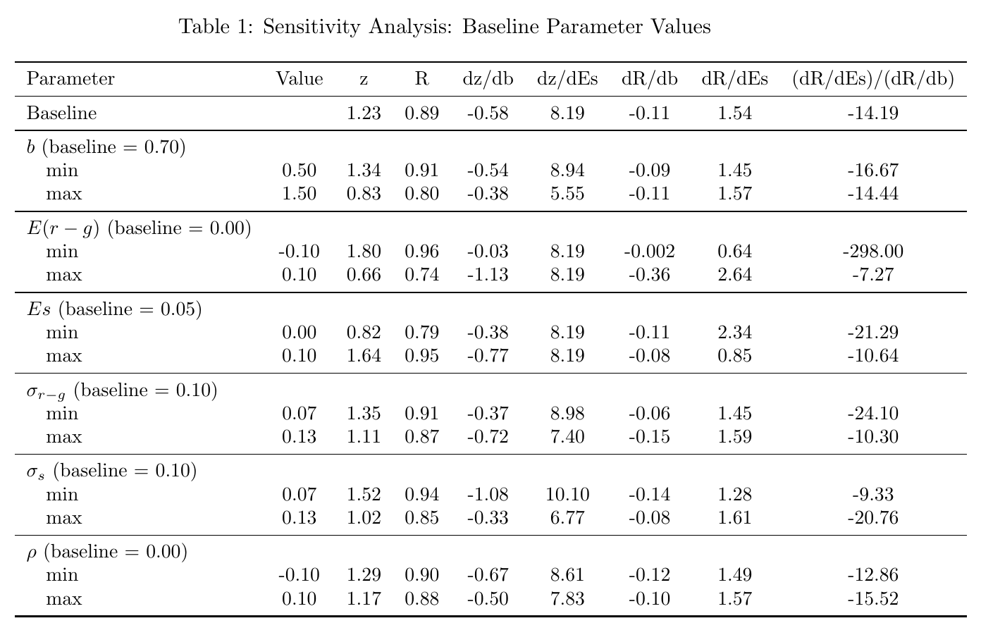
The number the paper cares about is in the last column of Table 1. The derivative of $z$ with respect to $Es$ is 8.19, and with respect to $b$ it is −0.58. The ratio of the rating effects is −14.19: a point of primary balance is worth about fourteen points of debt. The reason is visible in panel (a) of the schematic. The threshold stays put. A higher surplus moves the whole distribution away from it, while more debt only stretches the tail toward it. Raising debt from 0.7 to 1.5 (eighty points of GDP) takes the default probability from 0.11 to 0.20. Adding five points of cumulative surplus (one point a year) takes it from 0.11 to 0.05. Across the paper’s sensitivity rows the ratio runs from −7.27, when r − g is two percent a year, to −298, when r − g is minus two percent a year and debt hardly matters at all. The authors summarise it as “typically above 10 in absolute value.” That is the benchmark. Keep an eye on the threshold, though, because we will come back to it.

The model also makes two other predictions. Since r − g decides how much debt matters at all, a fall in r − g should make ratings noticeably more forgiving of debt. And country differences are allowed, but they are supposed to live in $x$: the investor base, the politics, whether the central bank is likely to step in.

What the agencies actually do

The empirical side takes 35 advanced economies from 1995 to 2025 and 97 emerging and developing economies from 1997 to 2025. S&P, Moody’s and Fitch ratings are mapped to an eleven-point scale, from 11 for AAA down to 2 for BBB−, and everything below investment grade is lumped together as 1. The authors estimate an ordered probit of the rating on lagged debt and on the forecast primary balance, which is the mean of the spring-WEO forecasts for years $t$ through $t+5$, with country and year fixed effects. The latent index plays the role of $z$. The country fixed effect plays the role of $x$. The headline statistic is the ratio of the primary-balance coefficient to the debt coefficient, set against Table 1’s −14.

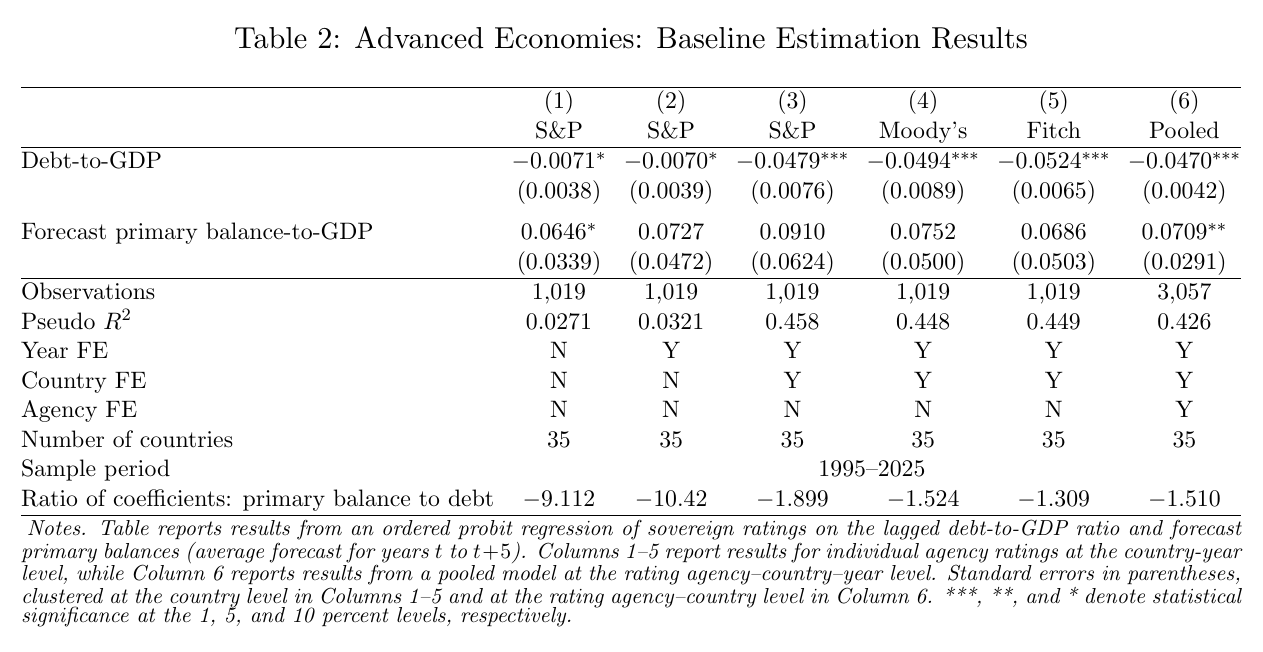
In the preferred specification, column 3 for S&P, the debt coefficient is −0.0479 and precisely estimated. The forecast primary balance gets 0.0910, which is not significant, and the ratio is −1.90. Moody’s gives −1.52, Fitch −1.31 and the pooled model −1.51. The pooled column is the only fixed-effects column where the balance clears conventional significance. In English: a point of forecast surplus, sustained over the six forecast years, buys the rating you would get from having about two points less debt. The model said fourteen.

One thing in the table deserves more attention than the paper gives it (this is our reading). Without country fixed effects, in columns 1 and 2, the ratio is −9.1 and −10.4, which is almost exactly the model’s neighbourhood. Adding country effects raises the pseudo-R² from about 0.03 to 0.46, which the paper reads as “country effects are important,” and fair enough. But it also multiplies the debt coefficient by about seven. Across countries, the agencies weigh debt against deficits roughly the way the model says they should. Within a country, over time, debt is what moves the grade. We return to what drives that within-country variation below.

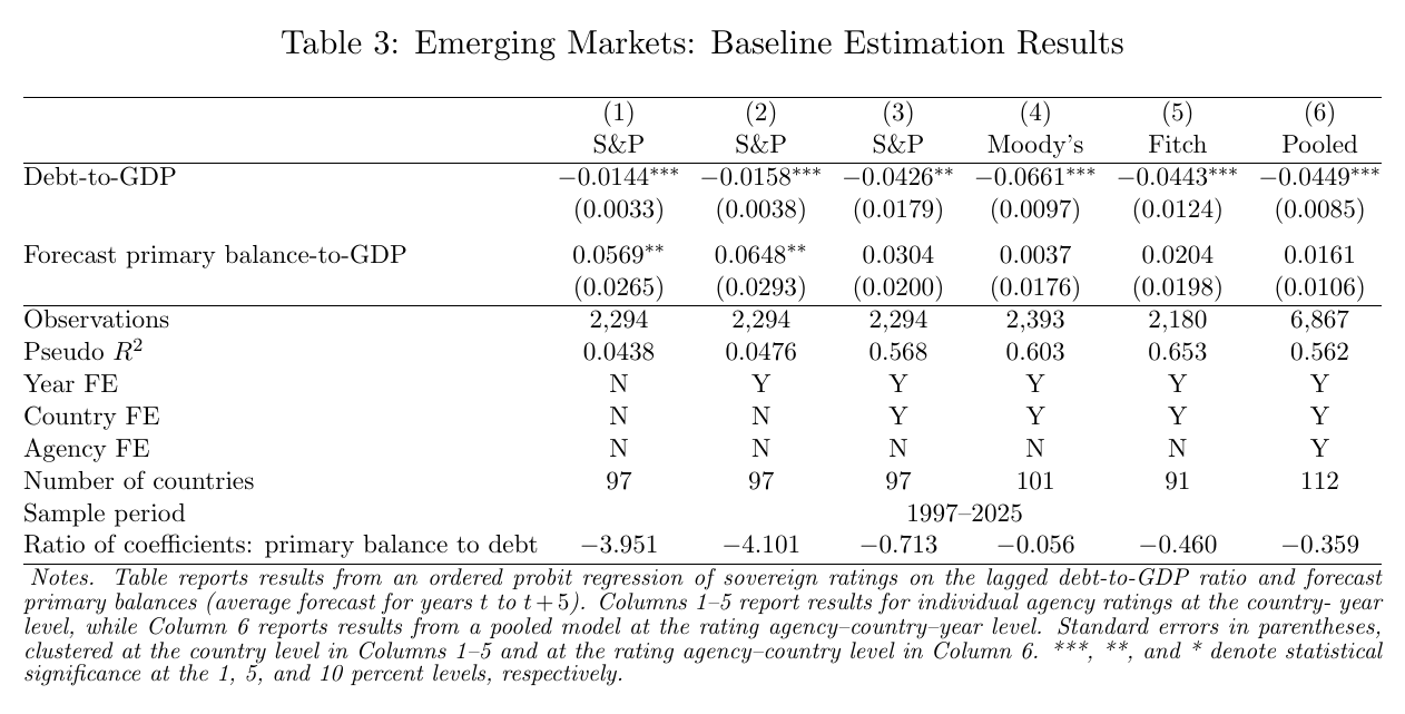
The emerging-market results in Table 3 are starker. The S&P ratio is −0.71, Fitch −0.46 and pooled −0.36. Moody’s puts a coefficient of 0.0037 on the forecast primary balance, for a ratio of −0.056. As far as that regression can tell, Moody’s does not look at the forecast at all. The authors flag the twist: emerging economies have lower r − g, which in the model makes debt matter less and should push the ratio up, and it comes out lower. (Keep the scale in mind too. 73 percent of emerging-market observations sit in the single junk bucket, so these regressions are mostly about crossing into investment grade.)

Maybe the forecasts are just bad

The obvious defence of the agencies is that the regressor is the IMF’s forecast, not theirs, and IMF fiscal forecasts are not famous for accuracy. If the agencies hold a better forecast and the WEO number is that forecast plus noise, the coefficient on the WEO number is attenuated and the ratio is biased toward zero. So the authors run a Mincer–Zarnowitz regression of realised average primary balances on the forecast, with lagged debt and both sets of fixed effects.

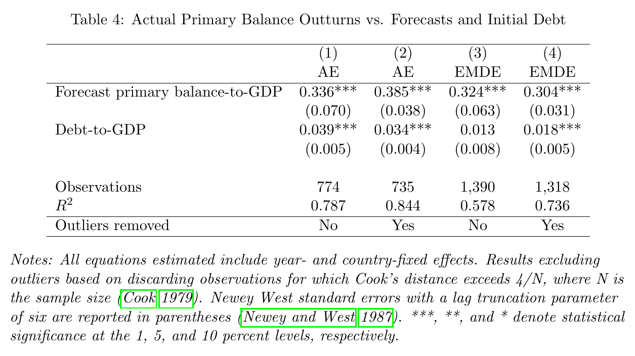
The slope is 0.336 for advanced economies and 0.324 for emerging ones, where rational expectations would give 1. Within a country, a one-point higher WEO forecast comes with about a third of a point more actual primary balance. Assume the agencies have rational expectations and the WEO forecast is their expectation plus white noise, and the true coefficient is the estimated one divided by that slope. The advanced-economy ratio goes from 1.3–1.9 to 3.9–5.7. The emerging-market ratio goes from 0.1–0.7 to 0.2–2.2. The paper calls this “closer to, but still well below” the model. It is a generous correction, too, since it gives the agencies the benefit of a forecasting ability nobody has shown they have.

The same table also has a debt coefficient that points the other way from what the authors worried about. Their second hypothesis was that forecasts get more optimistic as debt rises, which would push the debt coefficient in the ratings regression up in absolute value. What Table 4 shows is that, for a given forecast, higher debt comes with better-than-forecast outturns: 0.039 for advanced economies, significant, and significant for emerging economies only once outliers are dropped. The paper calls this “suggestive evidence, mainly for AEs” and leaves it there. On our reading, it is the opposite of the optimism story, and it amounts to a small, unnamed fiscal reaction function hiding in the forecast errors.

The r − g that didn’t register

The median advanced-economy forecast of r − g fell from about 2 percent in 1995 to about −3 percent in 2021 and has since come back to around −1 percent (partly, the authors note, because a lot of debt was locked in at low coupons). On the model’s logic, that should have made ratings much more lenient over time at given debt and deficits. The baseline year effects instead follow what the paper calls “a jagged path with some increase,” far from “the much stronger rising path … than would have been expected.”

To see what’s going on, the authors construct r − g from WEO forecasts, following Mauro and Zhou, for 27 advanced economies and 25 EMBI emerging markets. They let the debt coefficient vary with r − g and, in the most flexible version, with the year as well.

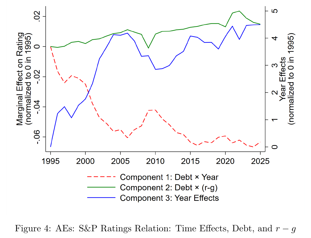
Figure 4 is the most interesting picture in the paper. Reading it by eye, the year effects (blue) climb by something like 4.5 latent units between 1995 and 2025, so at given fundamentals the agencies became much more generous. The debt-by-year interaction (red) falls by roughly 0.06, so each point of debt came to cost more. The authors’ comment: “We have no obvious explanation for this rotation.” Our back-of-envelope, not theirs: at mean advanced-economy debt of about 65 percent, the red line is worth about −0.065 × 65 ≈ −4.2 latent units, against roughly +4.5 from the blue. The two nearly cancel, and that is why the baseline year effects looked flat. Flat year effects did not mean nothing changed. Two large changes happened to offset each other.

The r − g contribution (green) creeps up by only a couple of hundredths. Its coefficient has the right sign and is significant at 1 percent in every column of Table A7, between −0.0024 and −0.0048, but in the paper’s words its effect is “much smaller than our theoretical model suggests.” The emerging-market version shows the same growing generosity in the year effects and the same harsher treatment of debt up to the mid-2010s, which then unwinds, and “no visible trend in the effect of r − g.”

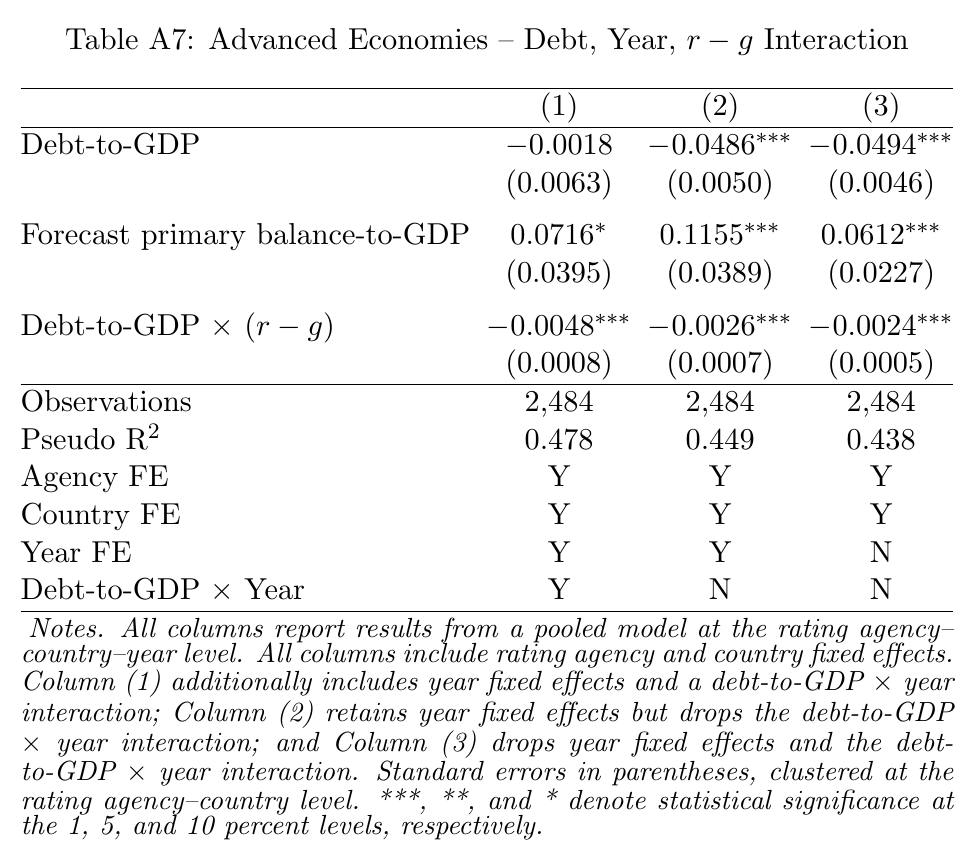
There is a way to read this that is kinder to the interaction and harsher on the debt level. This is our arithmetic, and it relies on the model’s $z$ and the probit’s latent index sharing a scale, which the paper asserts only loosely. Differentiating Table 1’s debt effect with respect to r − g gives an interaction of roughly −0.003 per point of debt per point of annual r − g, the same order as the Table A7 estimates. On that reading, the agencies respond to r − g about as much as the model says. What is out of line is the debt main effect itself, around −0.048 in the data against something like −0.006 in the model. A modest interaction cannot do much against a debt penalty that is already about eight times too large.

Who you are

Then there are the country effects, which the authors say “puzzle” them by their size. They translate them into two statistics. The first is the rating each country would get at common values of debt and forecast balance. The second is the “debt tolerance,” the debt ratio at which a country keeps an AA (9) with even odds, holding the forecast balance at zero and the year effect at its 2020 value.

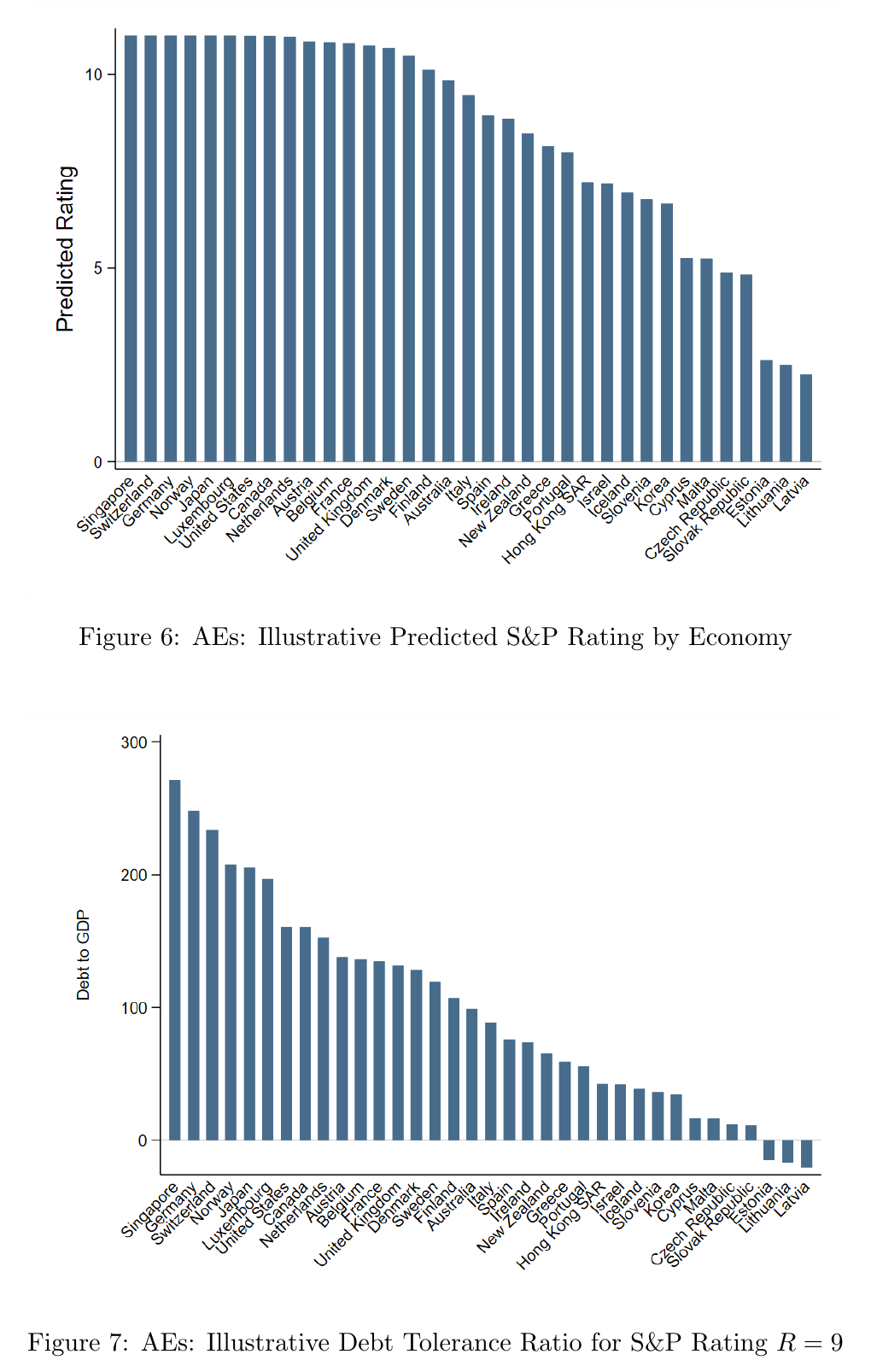
At the same debt and forecast balance, Germany gets 11, Ireland about 9 and the Baltic states about 2. On debt tolerance, Singapore can carry 272 percent of GDP and keep its AA, Germany 248, the United States 161, France 135 and Italy 89. For Estonia, Latvia and Lithuania the number is negative. Even at zero debt and a zero forecast balance, the estimates give them less than even odds of a 9. The emerging-market version is just as spread out: Qatar keeps a BBB− up to 161 percent, China up to 134, Mexico up to 79, and Pakistan, Argentina, Venezuela, Ukraine, Bangladesh, Türkiye and Nigeria are below zero.

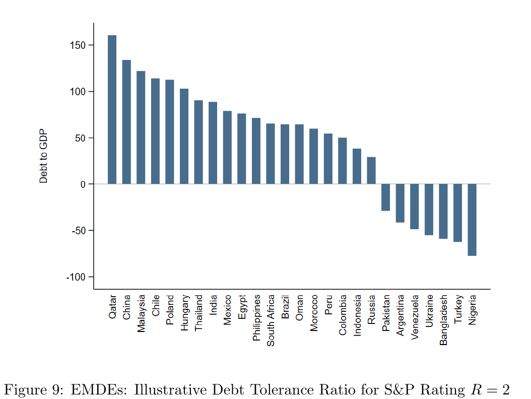
The authors grant that some of this is legitimate. Longer horizons, different uncertainty and different investor pools are exactly the country-specific $x$ the model allows for. But they judge the gaps “larger than can plausibly be explained by country-specific factors we have left out of our regression.” They are careful to say that the levels depend on the rating, probability and year chosen, while the cross-country differences do not. That is true by construction of a linear index, and it is worth knowing when you read the bars.

The conclusion is honest about where this leaves things: “It may be that our model is missing some essential aspects of the effect of fiscal policy on the probability of default. Or it may be that our model reaches roughly the right conclusions, and rating agencies should revisit their methods.” Hence “An Exploration.” In preliminary work, spreads put more weight on primary balances relative to debt than ratings do, “thus closer to the implications of our model, although a gap remains.” No numbers are given for that yet.

Our objections

The first objection is the one we care about most, and it is about the threshold we told you to keep an eye on. In the paper’s model, default is triggered by the change in debt, not its level. The authors say as much in footnote 5: “The natural assumption would be that default takes place if the debt ratio explodes over time,” and the five-year change rule is a concession to the WEO horizon. The concession is doing a lot of work. With r ≈ g and a change trigger, the level of debt enters only through the variance term in equation (3), so it has to matter little, and the large ratio is built in by the modelling choice. Look at panel (b) of the schematic, which is our variant and not in the paper. Default happens if debt ends the period above a fixed ceiling $\bar B$. Set $\bar B = b + x = 0.80$, which reproduces the baseline $z = 1.23$ and $R = 0.89$ exactly, with no fitting. Now ten extra points of debt move the threshold ten points closer, and the tail jumps from 0.11 to 0.35, where the paper’s fixed $x$ gives 0.12. By our arithmetic the ratio becomes about −0.93. It is close to −1 for any calibration, because under a level rule debt and the cumulative balance enter end-period debt one for one and the uncertainty channel adds only about 7 percent. One trigger makes the ratio large by construction and the other makes it about one by construction. The data cannot tell you which trigger is right.

Then there are units, which the paper sets out itself but never converts. In the model, $s$ is the five-year cumulative balance ($Es = 0.05$ “corresponds to an annual primary surplus of 1 percent a year”). The regressor is the annual average of six forecasts. So one point of the regressor is five or six points of the model’s $s$. By our arithmetic, the paper’s −14.19 is about −71 (or −85) in regression units. On the paper’s own benchmark, the gap between the model and the agencies is roughly five times bigger than reported. The level-trigger benchmark in regression units is about −4.7 to −5.6, which is uncomfortably close to the authors’ forecast-error-corrected advanced-economy range of 3.9 to 5.7. That closeness is mechanical (about −1 times five), and we would not make much of it. The point is that “are the agencies too debt-heavy” turns on a modelling choice the paper made for data reasons. Depending on that choice, the answer is either by an order of magnitude or hardly at all.

The second objection is about identification. With country and year effects, the debt coefficient is identified from within-country debt swings, and in this sample the large ones are bank bailouts, deep recessions and the euro crisis. At those moments ratings fall for reasons beyond the debt ratio: contingent liabilities, lost market access, politics. Lagging debt handles mechanical reverse causality, but it does nothing about an omitted crisis. The tell is the one noted above, a ratio of about −10 across countries and about −1.5 within them. The unexplained debt-by-year rotation in Figure 4 is also what you would expect if the within-country debt coefficient is partly picking up crises.

The third is about the country effects. The debt variable is presumably gross (the paper doesn’t say net), and the top of the tolerance charts is populated by exactly the sovereigns with large assets on the other side: Singapore, Norway, Qatar. A fixed effect is where net-asset positions would show up. Separately, in an ordered probit with a dummy for each country, a country that sits in one category every year is perfectly predicted, and its dummy is not pinned down, because the likelihood keeps improving as it drifts toward infinity. With 73 percent of emerging-market observations in the junk bucket and 37 percent of advanced-economy observations at AAA, this is not a corner case. A drift of three latent units moves a debt tolerance by about 3/0.0479 ≈ 63 points of GDP (our arithmetic). We have not checked which countries are single-category in the S&P data, or whether the estimation bounds the dummies. So the existence of big country effects looks safe, while the specific 248s and the negative numbers deserve less trust than the bar charts suggest.

Where that leaves you

Put the pieces together and the agencies do not look like a default calculator run on expected flows. They look like a rule that scores the stock, softened over time by a year effect nobody can explain and set, above all, by the country’s name. That may be the wrong rule. It may also be close to the level-trigger model, applied by people who never needed to write it down. The paper’s third proposed next step, looking at actual defaults, is the test that would separate the two, and it is the one the authors say they have not done yet. Until then, the cheapest way to raise your debt tolerance is to have been Germany for the last thirty years.