Optimal Time-Consistent Macroprudential Policy

Javier Bianchi and Enrique G. Mendoza, “Optimal Time-Consistent Macroprudential Policy.” This is the published version, in the Journal of Political Economy 126(2), 2018, pp. 588–634. There is no recorded talk and no discussant, so what follows is written from the published paper and its online appendix.

You own a piece of land. You would like to borrow. The bank is happy to lend, and it names a rule: you may owe up to 90 percent of what the land is worth.

Sit with the word “worth” for a second, because it is doing something strange. Your credit limit is not a number. It is a function of a price. And the price of land is not a fact about land; it is a fact about what people expect land to earn and how badly they want money right now. So your borrowing capacity is a claim on other people’s states of mind, and when their states of mind change, your credit line changes without anyone having lent or repaid anything.

Now make the observation that turns this from a fussy detail into a macroeconomics paper. Everyone has this contract. When the constraint bites, everyone sells land at once to raise cash. That pushes the price of land down. The price of land is what the credit limit is written on. So the credit limit falls, which forces more selling, which pushes the price down further. The bank did not tighten. Nobody made a decision. The contract simply re-priced itself downward using the consequences of its own enforcement as an input.

This is Irving Fisher’s debt deflation, and it is old. What Bianchi and Mendoza do is put it inside a calibrated general-equilibrium model, work out what a regulator would optimally do about it, and then — this is the part that makes the paper — discover that the regulator’s optimal plan is one it would not want to keep.

The model

There is one small open economy, one period is a year, and it is inhabited by a single representative firm-household — a creature that produces and consumes in the same body, which spares everyone an equity market. It produces with three inputs: its own labour, imported intermediate goods bought at a world price, and a physical asset in fixed unit supply. Call the asset land. Land is never built and never destroyed; it is only traded among domestic agents, which means its price is whatever the domestic Euler equation says it is. Market clearing is the single line $k_t = 1$.

The firm-household borrows abroad two ways. It issues one-period bonds at a world interest rate it takes as given. And it takes a within-period working-capital loan, at zero interest, covering a fraction $\theta$ of its input bill, paid before production happens. These are very different loans — one is a savings decision, one is a payroll float — and the paper’s central structural choice is that they draw on the same credit line:

That is equation (3), on p. 595. On the left, intertemporal debt plus the prepaid share of the input bill; on the right, a fraction $\kappa_t$ of the market value $q_t k_t$ of the land you started the period holding. The constraint binds only occasionally, and $\kappa_t$ itself flips between a loose regime of 0.90 and a tight one of 0.75, roughly the path of US mortgage loan-to-value ratios through 2008.

When the constraint binds, three things fire at once and all of them point the same way. Fire sales push the price down and the credit line with it — the Fisherian loop. Then, because the same collateral secures the payroll float, the effective cost of imported inputs jumps by a term proportional to the constraint’s multiplier, so inputs contract and output falls. This is a supply-side crisis, not merely a demand-side one, and it is the departure from the earlier literature where the constraint was written on a flow. And then the third thing, which is the second thing eating the first: because the price of land is the discounted stream of its future marginal products, an output collapse today and tomorrow lowers the dividends being discounted, which lowers the price, which lowers the credit line. A binding constraint hits collateral value twice — through the discount rate and through the cash flows.

The forward-looking price is what separates this paper from its ancestors. Because $q_t$ discounts an infinite stream, the mere expectation of a binding constraint at some future date raises expected returns and depresses the price today, in a perfectly tranquil year when nothing is binding at all. Your borrowing capacity right now is contaminated by beliefs about a bad year that has not happened and probably will not. Where borrowing capacity is instead a contemporaneous relative price, or a static fire-sale price, this channel simply is not there — and, as we will get to, neither is the time-inconsistency problem.

Why a planner would do something about it

The externality is the standard pecuniary one, and it is worth stating in the deflationary way. No individual agent is doing anything wrong. Each takes the pricing function as given, which is correct, because each is atomistic and does not move it. Each borrows a little more in a good year, which is individually optimal. It is just that the aggregate of all those individually correct decisions is a higher economy-wide debt state, which makes a binding constraint next year more likely, which lowers next year’s price, which shrinks everyone’s borrowing capacity in exactly the year they need it. Nobody internalises this because, individually, nobody causes it.

The paper is careful about the bookkeeping here, in a way that gets misquoted a lot. Relative to a frictionless economy, this economy underborrows — the constraint binds, and agents save precautionarily against it. Relative to a planner facing the same constraint, it overborrows. The pathology is not too much debt in the abstract. It is too much debt given that everyone else is also borrowing.

So put in a planner. Not a dictator: the planner cannot set the price of land. It chooses the bond position on the household’s behalf, subject to the resource constraint, subject to the same collateral constraint, and subject to the private asset-pricing Euler equation holding as an implementability constraint. That last one is what keeps the exercise honest. Prices stay market-determined; the planner just knows how its own borrowing moves them.

That is equation (12), p. 601: the value function, then resources, then the same collateral constraint the private agent faces, then the private pricing condition as a constraint the planner must respect. The calligraphic objects are the rules of future planners — consumption, hours, inputs, the multiplier, the price — which today’s planner takes as given, and which the Markov-perfect fixed point then forces to be identical to its own. The planner does not set $q$; it just knows the function.

The upshot is that the planner values a dollar more than the private agent does whenever the constraint binds, borrows less ahead of time, and can decentralise the whole thing with a state-contingent tax on debt, revenue rebated lump sum. The tax splits into a piece with a clean sign and a piece without one. The clean piece is what the authors label the macroprudential debt tax:

Equation (17), p. 605. Here $\xi_{t+1}$ is the multiplier on tomorrow’s implementability constraint, positive exactly when the collateral constraint binds tomorrow; $\mathcal{Q}$ is tomorrow’s pricing rule; and $u'' < 0$, which is what makes the whole ratio nonnegative — zero when nobody expects the constraint to bind, strictly positive otherwise. Provable, unconditional, no simulation required. It is the paper’s cleanest theoretical win, and it is worth noting that the closest comparable tax in the literature has an ambiguous sign. The other piece, present only when the constraint is already binding today, contains a term pushing toward a debt subsidy and another term of ambiguous sign, and the paper says plainly that combined they “can be positive or negative.” Hold on to that; it matters later.

And now the promise the planner will not keep

Here is the step that gives the paper its title. Suppose the planner could commit — pick the whole policy at date zero and be bound by it.

Ask what the committed planner would like to do in a crisis. It wants today’s land price up, because that is the credit line. Today’s land price is the discounted stream of tomorrow’s marginal utilities. Marginal utility is high when consumption is scarce. Therefore: promise scarcity. Announce that from tomorrow onward, consumption will be low. High future marginal utility means a high stochastic discount factor, which means a high price today, which means a looser constraint today and a smaller crash. The date-$t$ planner commits its successors to austerity purely as a price-support operation.

Then tomorrow arrives. The crisis is over. The price that the austerity was propping up is in the past and cannot be un-propped. Delivering the promised consumption cut now buys precisely nothing. Reneging is optimal.

This is visible in the algebra as a lagged multiplier that ratchets:

Equation (21), p. 608 — a positive, nondecreasing sequence that steps up every time the constraint binds and never steps back down. The stock of outstanding promises only grows, which is precisely why it cannot be a state variable in a well-behaved recursive problem and precisely why the plan is not credible.

The direction of this matters more than it first appears. The appendix’s illustrative example finds that the committed planner supports higher asset prices and higher debt than the unregulated economy — the opposite sign from the time-consistent planner, which holds prices and debt slightly lower in good times. Commitment is not prudential restraint with the volume turned up. It adds a second, noncredible instrument that leans the other way. So the authors set commitment aside and solve for the Markov-perfect policy, where the rules today’s planner assumes for its successors are the rules it itself would choose. Nested fixed point, value iteration inside, policy updating outside.

What comes out

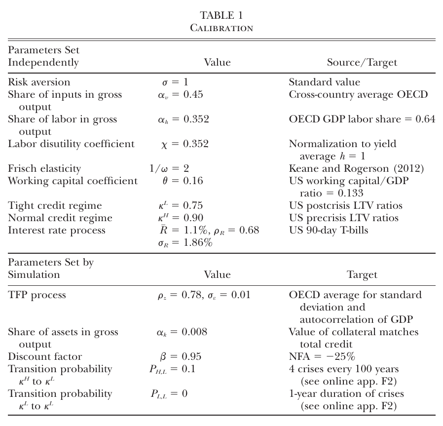
The model is calibrated annually to all 34 OECD countries, 1984–2012. Intermediates are 45 percent of gross output; the working-capital share $\theta = 0.16$ comes from total working-capital financing of 13.3 percent of GDP divided by a US intermediates-to-GDP ratio of 0.8; the world real rate averages about 1 percent with persistence 0.68. (The paper prints two different volatilities for that interest-rate process, one in the text and one in Table 1, and labels neither. They are plainly one estimated process in two conventions rather than two calibrations, but the source does not say which, so no volatility number appears here.) Crises are defined identically in data and model — a detrended current account more than two standard deviations above its mean — and the OECD data give a 4 percent frequency with a one-year duration against the model’s 3.8.

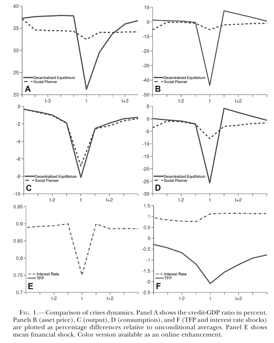
Then the clean experiment: simulate the unregulated economy for 100,000 periods, find the crises, and run the same shock sequences and the same starting debt through the planner’s policy functions, so both economies live the same history and differ only in who chose the debt. From four years out, the planner runs about three percentage points of GDP less credit than the unregulated economy. Three points. That is the entire intervention.

It buys this. Crisis probability falls from 4.0 percent to 0.02 percent. The asset-price collapse falls from 43.7 percent to 5.4. Consumption falls 26 percent in a crisis without the policy and 8 percent with it. Credit contracts by almost 18 percentage points of GDP between the year before the crisis and the crisis year, against 1.5 points under the planner. Output falls one to two percentage points more without regulation — the text says almost two, the printed figure reads closer to one — and that gap is the working-capital channel, the higher shadow cost of inputs when the payroll float is competing for the same collateral.

The nonlinearity is the point. From a common starting state, the unregulated economy ends a good year at a debt position of about $-0.245$ and the planner at about $-0.22$. A switch to the tight credit regime then forces the first to deleverage by roughly 700 basis points of GDP and the second by about 50. A two-and-a-half-point difference in debt produces a fourteenfold difference in the forced correction. This is an illustration at selected shocks rather than an event average, but it is the cleanest statement of why three points of GDP is not a small number here.

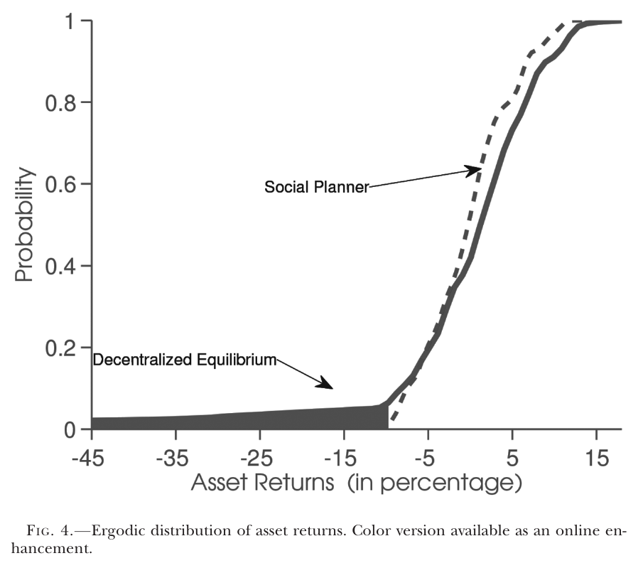
And the returns distribution grows a fat left tail out to about minus 45 percent, which the regulated economy does not have. The tail here is not a rare-disaster process bolted onto the shock structure. It is an equilibrium object: an occasionally binding constraint plus a feedback loop generates its own tail out of ordinary shocks. This is a rather nice thing for a model to do.

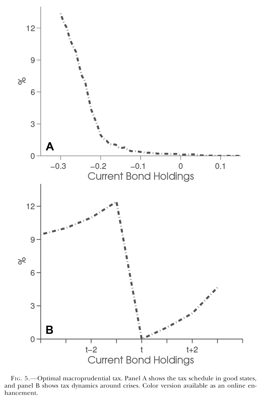
The tax itself averages 3.6 percent, correlates 0.7 with leverage, and — per the introduction, the text and Table 3, three statements against one — has a standard deviation about half that of GDP. (The conclusion on p. 630 says instead that the tax is “60 percent more volatile than output.” That sentence is inconsistent with everything else the paper reports, and appears to be an error.) The schedule reaches 13 percent at the most indebted states and is exactly zero in the safe region. Around a crisis it climbs for four years, peaks near 12 percent the year before, and goes to zero in the crisis year itself, because at that point the constraint is already binding and the probability of it binding next year is zero, so the prudential motive has nothing left to do. One caveat the paper is explicit about: what Figure 5 plots is the macroprudential component. In the crisis year, when the constraint binds, the full implementing tax carries that second, ambiguously signed component, and the paper does not show the total wedge to be zero.

The most quotable fact in the paper is a sentence about state-space geometry on p. 617. Under the optimal policy, crises are 0.02 percent events — and the region of the state space where the constraint is slack today but could bind tomorrow, the region where the macroprudential tax is levied, carries almost 94 percent of the planner’s long-run probability mass. The policy prevents crises essentially always by being on essentially always.

The welfare gain is 0.30 percent of permanent consumption, computed as the standard Lucas-style compensating variation and averaged over the unregulated economy’s ergodic distribution. That is a small-sounding number that the paper is right to call sizable, because the benchmark is small: the authors cite Lucas (1987) as having estimated a gain of “only 0.0005” from eliminating US business cycles, a sentence that carries no unit in the original, so it is best left un-arithmetic. The gain here is large by that standard, and the paper is candid that the absolute number is held down by the representative-agent, stationary-consumption structure. It is also emphatic about why it is not smaller: the gains are not only consumption smoothing. Cutting the working-capital parameter by a quarter, from 0.16 to 0.12, cuts the welfare gain by about a third, from 0.30 to 0.21 — a sensitivity to that parameter, not a decomposition of the total, but enough to show that the crisis is being valued as a hit to economic activity and not merely to consumption variance.

The surprising thing, which is about implementation

A regulator reads all this and does the obvious thing. The optimal tax averages 3.6 percent. State-contingent schedules are hard to legislate, hard to explain, hard to defend to a bank lobby. So: impose 3.6 percent, flat, all the time. Roughly optimal on average, vastly simpler, and surely a blunter version of the right policy.

It is not a blunter version of the right policy. It is worse than doing nothing, by a lot.

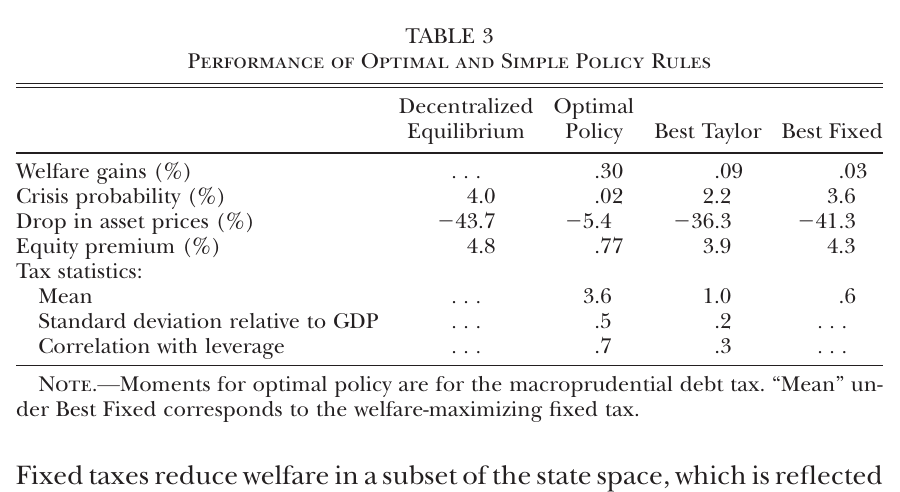
The welfare-maximising fixed tax is 0.6 percent — one-sixth of the optimal policy’s mean — and it delivers an average gain of 0.03 percent, one-tenth of the optimal policy’s 0.30. Raise the flat tax above 1.2 percent and the average welfare gain turns negative. Push it to 2 percent and the worst-affected state loses 1.5 percent of permanent consumption. The minimum welfare gain is negative for every fixed tax the authors try. And under the best fixed tax, Figure 8 shows crisis dynamics that are, in the paper’s words, “about the same as in the unregulated DE.”

The mechanism is exactly the one the whole paper is built on, turned against the regulator. A debt tax makes bonds expensive relative to assets, which shifts portfolio demand from assets toward bonds, which depresses the price of assets. The price of assets is the collateral. So a permanent debt tax permanently depresses collateral value — including in the crisis states where collateral value is the only thing that matters. There is an offsetting second-order benefit, because the tax makes assets less risky, and it is dominated. The optimal policy escapes the trap because it is state-contingent: its macroprudential component goes to zero in the crisis year, so the prudential levy is never applied at the moment when applying it would tighten the very constraint the levy exists to loosen. What the paper establishes is the scoreboard — 0.30 against 0.03 — not a decomposition of where inside the policy that difference is generated.

This is genuinely non-obvious, and the paper says why. In Bianchi (2011), the closest antecedent, fixed taxes are a crude version of the optimal one and not harmful. The reversal here comes entirely from the forward-looking asset price, which is exactly the ingredient this paper added. A middle option does exist: a “macroprudential Taylor rule” that makes the tax an isoelastic function of the debt position relative to a target, with the elasticity and the target found by numerical search rather than estimated. The best one — elasticity 2, target 200 basis points below the unregulated average debt — halves the crisis probability to 2.2 percent and earns 0.09 percent, about a third of the optimal policy. Simple rules can work. They have to be designed on purpose, and other parameterisations of the same rule are, the authors note, “significantly inferior.”

What a referee would push on

There was no discussant and no recorded Q&A, so the following is the case a referee would make and what the paper has to say back to it, drawn from its own text and appendix rather than from anything that happened in a room.

The first question writes itself: time inconsistency is your title, and you never solve the commitment problem in the calibrated model, so nobody can see what it costs. Conceded, and in the paper’s own words — “A comprehensive analysis of this issue is beyond the scope of this paper.” Appendix E gives the ratchet proof and an illustrative example on a stripped-down model with linear technology, TFP shocks only, and coarse grids. There is no number for the welfare cost of the commitment gap. The Markov policy delivers 0.30 percent; whether the Ramsey planner would have delivered 0.35 or 3.0 is unknown. The implicit defence — the commitment policy is irrelevant precisely because nobody would believe it — is a good answer to a policy maker and a thin one to a referee, who wants to know the size of the prize.

Second: your planner is a benevolent, perfectly informed dictator over aggregate debt; is a debt tax really the same object? Mostly yes, and the paper works at it. Proposition 1 does the decentralisation, and the appendix shows the same allocations and the same taxes arise if the planner is modelled as choosing taxes under discretion against competitive equilibria. It also handles the awkward case where the optimal total tax would be negative, by imposing nonnegativity — though here the main text’s claim that the macroprudential tax has “the same form” is a compression: the appendix’s own result carries the familiar externality term plus an extra term from the possibly binding nonnegativity constraint on future tax rates. On information, the appendix runs an early-warning exercise on a half-million-period simulation and finds that a logit on credit-to-GDP alone does roughly as well at flagging crises as knowing the true model — though the design fixes a common probability cutoff rather than a common error rate, so the achieved error rates differ across methods and should not be quoted as matched. What is not addressed is that the regulator here observes the debt position and every shock exactly, and has unlimited lump-sum fiscal capacity. The paper cites its own related work as evidence that informational frictions “can significantly affect” effectiveness, which is a promissory note.

Third, and this is the objection the paper visibly worked hardest on: Jeanne and Korinek studied the same externality and got a much weaker policy. Which of you is right? The answer comes in two separable pieces. On calibration, their constant term dominates their constraint, so only 7 percent of borrowing capacity depends on asset values — the Fisherian loop is switched almost off by construction, and their exogenous output makes crisis probability policy-invariant. Their optimal tax cuts the crisis price drop from 12.3 percent to 10.3; here it goes from 43.6 to 5.4. On formulation, their planner takes a reduced-form pricing function as given, so borrowing capacity today is predetermined with respect to today’s debt choice — and the appendix proves the two planning problems are not equivalent in either direction, shows their key assumption can fail under the CRRA utility both papers use, and constructs counterexamples where their planner is structurally forbidden from the higher-welfare debt choice. The residual a referee keeps: checking that assumption requires the true Markov pricing function, which you have to solve for first, as the authors concede; and the counterexamples do not establish that the quantitative gap is due to formulation rather than calibration, since both differ.

Fourth: land is not traded internationally and cannot be accumulated, and both assumptions are load-bearing. The paper flags the first itself, which is to its credit — with frictionless foreign trading, the asset is priced by world-rate discounting and the domestic constraint stops moving it, which guts the mechanism entirely. The defence, that with trading costs prices respond and the conclusions survive, is asserted rather than shown, and a footnote concedes the optimal policy would then also acquire a terms-of-trade motive. On accumulation, the appendix sets up investment with adjustment costs and Mendoza (2010) is cited for amplification surviving capital accumulation.

Fifth, and most consequential for the headline number: fixed asset supply, one-period debt, one representative agent — the crisis is mechanically too violent. Flagged twice, unprompted, which is the right instinct. A footnote concedes that “the model produces large credit drops partly because all intertemporal credit is in the form of one-period bonds, whereas loans in the data have, on average, a longer maturity,” and the Great Recession experiment in the appendix overshoots the observed current-account reversal for the same reason. Since the welfare gain is essentially the value of not having the crisis, anything that makes the crisis too severe inflates the 0.30 percent. There are also no intermediaries, no heterogeneity, no default, no nominal contracts and no monetary policy; the conclusion lists all of these as the agenda.

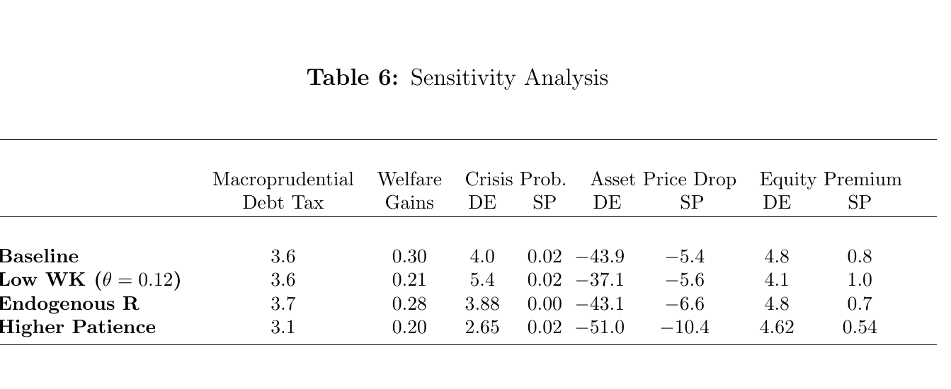
Sixth: how much of this is the working-capital bell you added? The paper answers with the sensitivity above and nothing stronger — cutting the parameter by a quarter cuts the gain by about a third. That is a derivative, not a channel share; working capital is still in the model in the low-$\theta$ row. It reads more as a defence than a weakness, since the supply-side channel is precisely why this paper gets 0.3 percent where consumption-smoothing-only exercises get Lucas-sized numbers. But the channel is calibrated off a single US 2013 cross-section and applied to an OECD-wide model, and anyone quoting that row should notice that crisis probability moves the wrong way when the parameter falls, from 4.0 to 5.4, and work out why before using it.

Seventh, the one that will make a referee squint hardest: you set the exponent on collateralisable assets to 0.008 so that the constraint binds at the mean. Is that not assuming the answer? The paper is transparent about it — the observed capital share accrues to the whole capital stock, not to the fixed-supply collateral asset, so the parameter is set instead to make the constraint hold with equality at unconditional means in the tight credit regime, and a footnote reports that a deterministic-steady-state alternative gives 0.012. Transparency is not the same as an answer. The parameter governing how much collateral exists is chosen to match observed leverage, which is the same object the amplification mechanism then operates on.

And eighth, the one the paper answers best by conceding: is the overborrowing result general? No, and it says so. Under other parameterisations the two bond rules can be close, and “there can even be instances in which the DE chooses higher $B'$.” Likewise the total optimal tax has ambiguous sign whenever the constraint binds; only the macroprudential component is provably nonnegative. And the 0.02 percent crisis probability under the policy is a threshold-defined statistic, computed with the unregulated economy’s crisis thresholds in levels. Restandardising raises it, though not remotely to 4 percent.

Anyway

The finding underneath all of this is not really “regulate credit booms,” which everyone already believed, and it is not really the 0.30 percent, which is a small number attached to a lot of modelling assumptions. It is that the shape of the policy carries almost all of the value, and the shape is counterintuitive in a specific way: the instrument has to be on almost all the time and off at exactly the wrong-seeming moment, because the thing it taxes is also the thing it is protecting. A tax on debt is a tax on collateral demand. Apply it in the crisis and you are tightening the constraint you built the tax to loosen.

Which puts a real regulator in an awkward position, because the political economy of macroprudential policy runs the other way entirely. Nobody wants to raise the debt tax in year seven of a boom when nothing is visibly wrong, and everybody wants to be seen doing something in the year the prices crash. The paper’s planner does the opposite on both counts. It is also, by construction, a planner that cannot commit — and the reason it cannot is that its ideal plan is a promise of future austerity made purely to hold up today’s asset prices, which is a sentence you could have found in a central bank speech at almost any point in the last fifteen years, usually delivered as a virtue.