Borrowing for Breakthroughs: Student Loans and Innovation

Alex Bell and Vikram Jambulapati
Presented by Alex Bell at the nber Economics of Talent Conference, Cambridge ma, 2 October 2026 (video). No discussant.
Source note: the paper version used is the preliminary conference draft dated 18 April 2025, posted for the nber conference. The talk is about eighteen months newer than that draft. The elasticity, the benchmark comparisons, the heterogeneity cuts and the citation-quality table appear only on the talk’s slides; the draft lists citation quality and heterogeneity as future work. Each number below says which of the two it comes from.

Two stories about debt, one of which has to lose

Student loans and innovation have two stories, and economists believe both of them. In the first, a loan buys you more and better schooling, and lets you spend your sophomore year in a lab instead of behind a register. More human capital, more patents later. In the second, the loan is a liability with a repayment schedule. You graduate owing money, and the career that pays off in social spillovers and a lottery ticket loses to the one that pays a salary. Bell’s own version of the second story, from the talk (02:28:17): “should I really be going into, you know, innovation, the sort of risky career with social spillovers, or do I want to go into banking where I can actually make enough money to to repay my student loans?”

The second story is debt overhang, and it has a decent empirical record. The draft cites Rothstein and Rouse (2011) on public-interest jobs, Field (2009) on the nyu Law aid experiment, and Krishnan and Wang (2019) on entrepreneurship. All of them find debt pushing people away from the socially useful, privately unrewarding path. And the draft’s own descriptive section makes overhang look even more plausible for inventors. It finds no sign of large private returns to the average invention: credit scores and credit-card balances, if anything, grow more slowly after someone files a patent (paper p. 9). If inventing doesn’t pay you, a loan bill is exactly the thing that should talk you out of it.

So the question is which story wins at the margin. The answer here is human capital, by a lot, for the people the experiment can see.

The kink tells you who is constrained

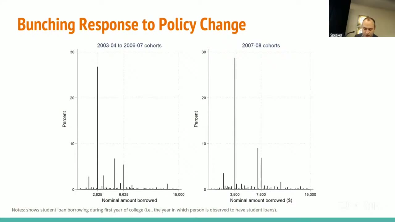
The design comes from Black et al. (2023), and it turns on a credit constraint you can see. The federal Stafford loan caps how much a dependent first-year undergraduate can borrow. Through the 2006-07 entry cohort the cap was $2,625. The Higher Education Reconciliation Act raised it to $3,500 for 2007-08 entrants. Then the Ensuring Continued Access to Student Loans Act raised it to $5,500 from 2008-09 on (paper p. 5; Table 2).

The histogram is the whole identification strategy in one picture. A large share of first-year borrowers sit exactly at the cap, and when the cap moves, the spike moves with it. Nobody’s optimal loan is exactly $2,625 by coincidence. Bunching at a statutory limit is a borrower telling you, in the only way the data allow, that they’d have taken more if allowed. So the paper calls a borrower “constrained” if, before the change, they borrowed exactly $2,625, or, after it, anything between $2,625 and their cohort’s new cap (footnote 5, p. 10). Everyone else who borrowed is the comparison group. The design is then a difference-in-differences: how did the constrained borrowers’ later patenting move, relative to the unconstrained, when the cap was lifted on them?

The data are the hard part, and Bell was cheerful about it. Inventors come from uspto records, covering grants and published applications. They are linked by an anonymised “hashed merge” (“if you don’t know what a hash merge technique is, good, stay that way” (02:29:33)) to the University of California Consumer Credit Panel. That panel holds quarterly credit-bureau records for 2004–2021, covering every Californian with a credit file plus a 2 percent national sample, and it keeps following people after they leave the state. The result, per the draft, is almost 250,000 inventors who ever lived in California, about a third of all us inventors (p. 3). The credit file has no enrollment records, so the year you started college is defined as the academic year of your first student loan (p. 6). That makes the sample first-year borrowers only. Whatever the loan cap does to whether people go to college at all, this design can’t see it.

Bell flagged up front that this is a late, and that he expects it to be a big one (02:30:38). First, there’s Roy-model selection: a student who “kind of can’t afford college but decides to go to college anyway” may know something about how high their returns are. Second, the episode is from the early 2000s, when the misallocation of talent in Hsieh et al. (2019) was plausibly worse than it is now. A presenter who tells you in advance why his estimate is probably too large for today’s policy is a presenter worth listening to.

The specification

The main difference-in-differences regression (paper eq. 2):

Here $y_{ic}$ is patent filing (per 1,000) for borrower $i$ in entry cohort $c$, where $c$ is the spring year, so 2005 means 2004-05. $\delta_c$ is a cohort fixed effect, and $\beta_2$ is the effect of having your constraint lifted.

To turn that into a per-dollar number, the draft follows Black et al. and instruments first-year borrowing with the same interaction (paper eq. 3):

$\mathit{Loans}_{ic}$ is first-year borrowing in thousands of dollars, so $\beta_2$ is the effect on patenting of one more $1,000 of first-year debt. (The slide version of the first stage, at 02:35:54, writes the instrument as constrained interacted with each cohort dummy rather than with a single post indicator. Neither source says which version produced the table below.)

The first stage works as you’d hope. Constrained borrowers’ first-year debt rises by about $680 relative to the unconstrained in the 2007-08 cohort, whose cap rose $875. It rises by more than $1,700 in later cohorts (paper p. 11, Figure 6). Those later cohorts’ cap rose by $2,875, from $2,625 to $5,500; the draft says “$2,500”, which is a slip. Pass-through is well below one because not everyone borrows up to the new cap.

Patents go up, and OLS doesn’t see it

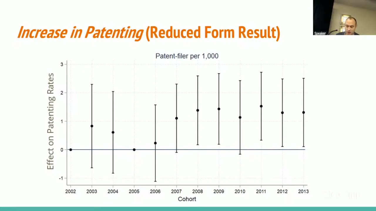
The reduced form is roughly one extra patent filer per 1,000 constrained borrowers from the 2007-08 cohort onward (paper p. 12). Look at the picture honestly. The pre-period is not a flat zero: 2003 and 2004 are positive and noisy, with intervals as wide as the post-period’s. And the 2007 dot, the first cohort with a higher first-year cap, has an interval that dips just below zero. What the picture supports is a level shift in the later cohorts, measured with plenty of noise.

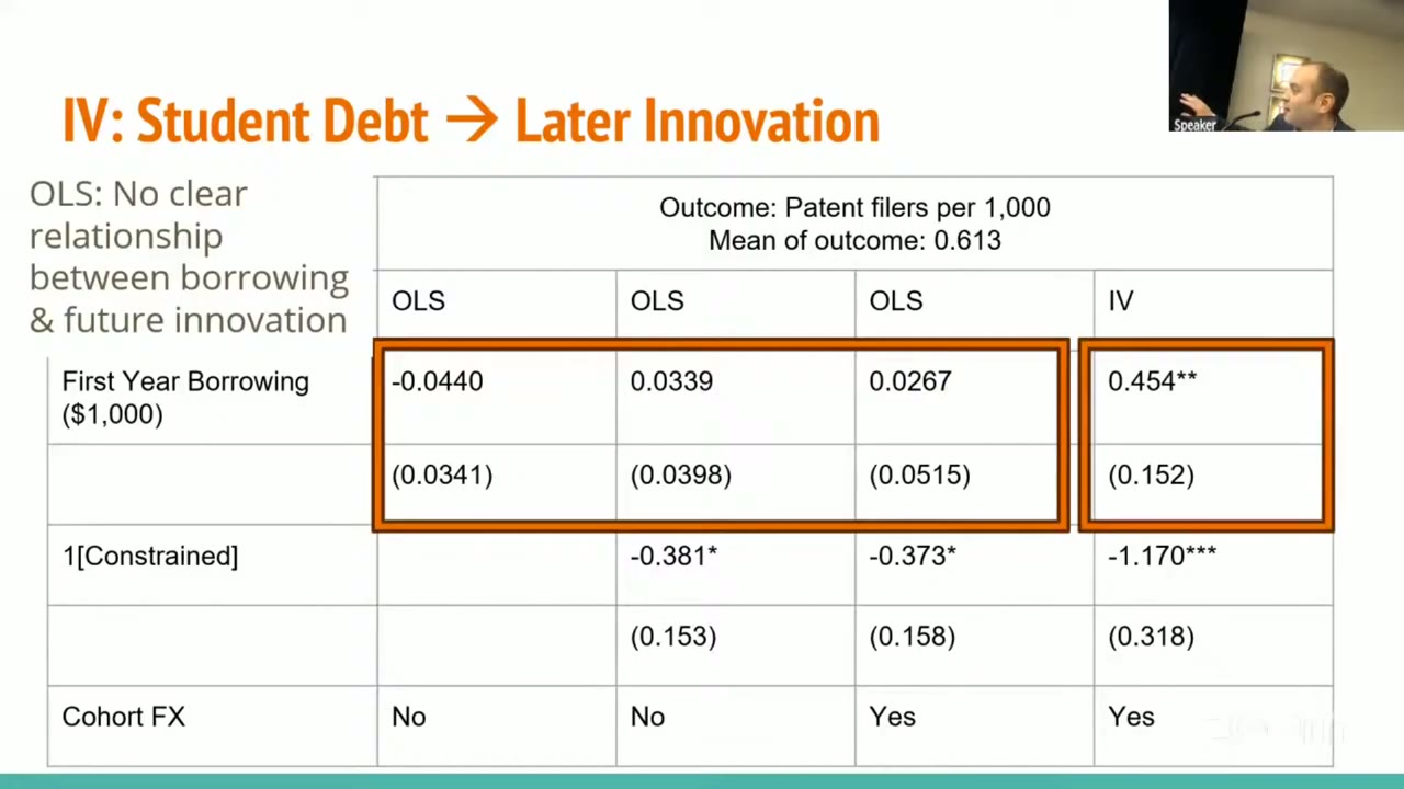
The ols-versus-iv contrast is where the paper earns its keep. Naive ols says student debt and later patenting have nothing to do with each other; column (1)’s point estimate is even slightly negative. The draft calls that 6.7 percent of the mean, though 0.044/0.613 is closer to 7.2. The iv coefficient is 0.454 more inventors per 1,000 for each extra $1,000 of first-year debt, on a base of 0.613. The draft calls that “approximately a 73% increase” with a lower bound of 25 percent (p. 12). The talk says 74 percent, which is the correct rounding of 0.454/0.613, and restates it as innovation rates moving “from 61 to 107 inventors per 100,000” (slide at 02:36:39). In Bell’s words, “a very small number to another very small number. That’s actually bigger in percentage terms” (02:36:42).

The ols null is not puzzling once you remember who borrows. The draft notes that innovation rates are clearly lower among constrained students than unconstrained ones (p. 12), and the slide’s $\mathit{Constrained}$ row says the same in levels. Heavy first-year borrowers plausibly come from poorer families, the margin along which the lost-Einsteins literature finds less inventing (that link is my gloss, not the authors’). So the cross-section likely carries selection running against debt, and the cap change is what lets you see past it.

How big is 74 percent? The slide-only part

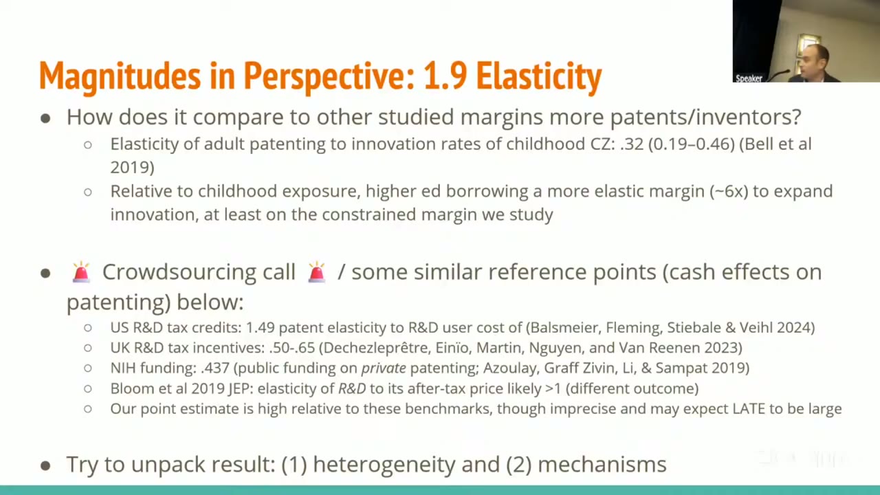
None of what follows is in the April 2025 draft. In the talk, Bell converts the iv estimate into an elasticity of patents to loans of 1.9, with a confidence interval of .67 to 3.22 (slide at 02:36:39), “basically just dividing through by the mean loan rate” (02:37:31). More precisely, it’s the 74 percent scaled by the mean first-year loan over $1,000. Neither source reports that mean. Backing it out from 1.9/0.74 gives roughly $2,570, which is my arithmetic, not theirs. The slide calls 1.9 “very similar” to the elasticity of Stem degree completion in Black et al. (2023).

Then come the benchmarks. Against his own earlier work, the elasticity of adult patenting to childhood commuting-zone innovation exposure (.32), student borrowing comes out about six times as elastic. That’s a ratio of point estimates. The two intervals (.67–3.22 and .19–.46) would let the true ratio be anything from about 1.5 to about 17. The other reference points are R&D tax credits in the us (1.49) and uk (.50–.65) and nih funding (.437), and Bell billed them as a crowdsourcing call rather than a finished comparison. His own summary is the right one: “our point estimate looks somewhat high relative to these benchmarks … although it’s an imprecise estimate with a wide confidence interval” (02:39:18). The heterogeneity cuts by imputed gender, imputed race and technology class are also slide-only, and he dismissed them in one breath: “we just can’t get a lot of significant differences there” (02:40:00).

Lost Einsteins, or lost tinkerers?

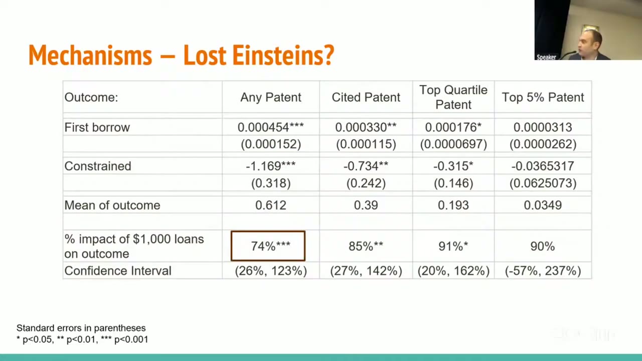
The obvious deflationary reading of a 74 percent jump in a very rare outcome is that the loan cap is producing marginal patents: the defensive filing, the incremental claim. The slide-only citation table tests this by re-running the iv with progressively pickier outcomes. Citations are ranked within grant year so that recent patents aren’t penalised for being young. If the marginal inventors were low-grade, the percentage effect should shrink as the bar rises. It doesn’t: 74 percent for any patent, 85 for a cited patent, 91 for a top-quartile patent, 90 for a top-5-percent patent. (The coefficients are per dollar, so 0.000454 is the same 0.454 per $1,000 as before.)

But read the bottom row before you get excited. The intervals overlap almost completely, (26, 123) against (20, 162), and the top-5-percent effect is not distinguishable from zero, (−57, 237), because its base rate is about 3.5 per 100,000. (The slide also gives the headline coefficient three stars; at 0.454/0.152 ≈ 3 it is the two-star result the draft’s Table 3 reports.) Bell stated it at exactly the right strength: “no evidence that these uh marginal innovations are of any lower quality … if anything, the point estimates seem to suggest they’re higher quality, but there’s no real statistical significance behind that statement” (02:41:42). So this is absence of evidence that the extra inventors are worse. It is not evidence that they are Einsteins.

The cohorts that got treated before their cap moved

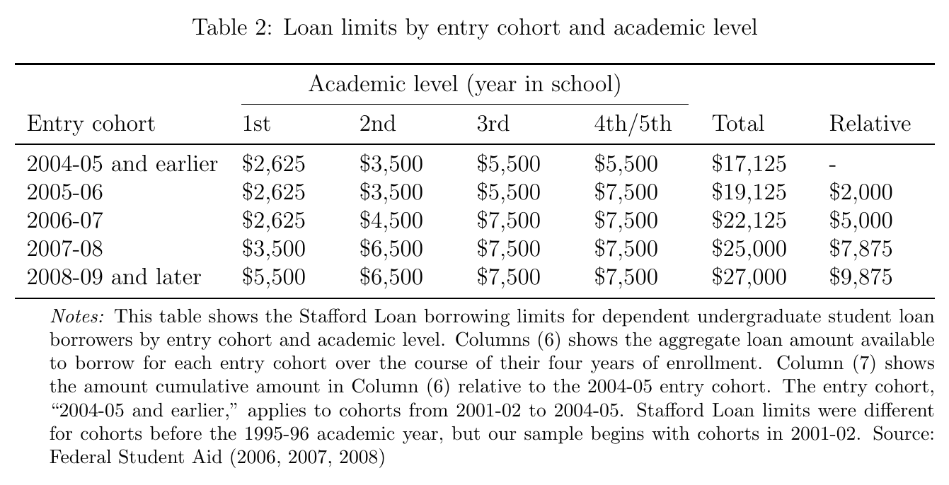
Here is something nobody raised in the room. It is my own reading of the draft, not a point the authors make. Equation 2 codes every cohort after 2005 as “post”, which includes the 2005-06 and 2006-07 entrants. Their first-year cap never moved, and their first-stage effect is about zero. They were treated anyway, later in college. Table 2 shows their four-year borrowing capacity up $2,000 and $5,000, because the sophomore-and-up limits rose underneath them. So the instrument shifts total borrowing over the degree, not only the first-year loan that the iv divides by. If later-year borrowing also matters for patenting, the exclusion restriction (instrument affects patents only through first-year loans) may be violated. Scaling by first-year debt alone would then overstate the per-dollar effect. The event-study dots for those two cohorts are too noisy to settle it either way. The fix is cheap: drop them, or code them as pre, and see whether 0.454 survives.

Two more draft-level caveats. The sample is first-year borrowers, so the extensive margin of college entry is invisible. And “unconstrained” means everyone else who borrowed, a group whose composition the draft doesn’t describe.

What the room asked

The Q&A lasted about seventy-five seconds, squeezed in while the next speaker set up, and nobody went after the identification. An unnamed questioner asked whether the effect comes from students switching into Stem or from studying more overall (02:43:28). Bell said the credit data can’t answer that, since they have no major or enrollment fields: “it’s really hard in this data to get into the mechanisms.” He offered the hypothesis the team started with: a student who doesn’t have to work through school “might have more time to be sort of creative, flexible, explore the topic” (02:43:40). A second question, mostly lost in the audio, was about timing, either when the patenting shows up or whether any shows up during school. Bell said the estimates are “a little bit too imprecise to do a lot on the timing”, and that pushing further might show whether “it turns to mush” (02:44:11).

His closing update was more careful than his headline. The early-2000s reforms “probably look like they have uh had quite a lot of value in uh producing innovation among the students that were impacted”. But on what a cap increase would do today, he has “a more diffuse prior”, because it depends on who the marginal borrower is now (02:42:13). That’s the right place to land. Policy debates mostly treat student debt as a liability problem. This paper’s best guess is that, for the students pinned at the cap, the scarce thing was the right to borrow more, and the debt-overhang problem turned out to be the smaller one.

References