The Long-Run Risks Model and Aggregate Asset Prices: An Empirical Assessment

Jason Beeler and John Y. Campbell, Critical Finance Review 1 (1), 2012, pp. 141–182. Version used: the October 2011 author version, with its online appendix; no recorded talk.

Beeler and Campbell’s paper is the long-run risk model’s most thorough audit, and its method is to take the model at its word. The model’s central object is a small, persistent drift in expected consumption growth, $x_t$, that you cannot find in consumption data. Bansal and Yaron (2004) are candid about this, and they have an answer: the econometrician cannot see $x_t$, but investors can, and they price it. Fine. But if investors price it, then prices contain it, and you can get it back out of prices. The log price–dividend ratio becomes the model’s own window onto the thing the consumption data won’t show you. So if the model is right, the price–dividend ratio should forecast long-run consumption and dividend growth. It should also forecast everything else the model’s hidden states forecast.

That is the whole paper, done once for growth, once for volatility, once for real bonds and once for the elasticity of intertemporal substitution. The model is checked against two calibrations: Bansal and Yaron’s original (by), and the recalibration by Bansal, Kiku and Yaron (bky), which the October 2011 version cites as a 2011 working paper. The answer, roughly, is that prices know a great deal about future returns, something about future consumption volatility, and almost nothing about future consumption growth. That is close to the reverse of what the model needs.

The mechanism: one price, two hidden states, and a dial

The endowment is four lines, at a monthly frequency:

This is eq. 1 in the paper: $x_t$ is the persistent component of consumption growth with persistence $\rho$, $\sigma_t^2$ is the conditional variance with persistence $\nu$, mean $\overline{\sigma}^2$ and shock scale $\sigma_w$, $\phi$ is the leverage of dividends on $x_t$, $\varphi$ is the dividend volatility multiple (not to be confused with leverage), and $\pi$ is dividends’ exposure to the consumption shock $\eta$.

The investor has Epstein–Zin (1989) preferences with an eis $\psi$ of 1.5 and risk aversion $\gamma$ of 10. eis above one makes stock prices rise with expected growth and fall with volatility, and eis above $1/\gamma$ makes news about the future priced, not just the current consumption shock. Solve with the loglinear Campbell–Shiller (1988) approximation, with the linearisation constant solved as a fixed point rather than assumed (the authors insist on this, and bky use a similar analytical solution), and the price–dividend ratio comes out as

This is eq. 3 in the paper: $z_{m,t}$ is the log price–dividend ratio of the dividend claim, and $A_{1,m}$ and $A_{2,m}$ are its loadings on expected growth and on variance, positive and negative respectively under these calibrations.

Eq. 3 is not an extra assumption. It is the solution. And it says something very restrictive: the one valuation ratio you can observe is a linear combination of the two states you can’t. Whatever $x_t$ forecasts (future consumption and dividend growth), and whatever $\sigma_t^2$ forecasts (future consumption volatility, future dividend volatility, future return volatility), $p - d$ has to forecast too, in proportions fixed by the loadings. The calibration decides how much of the ratio each state accounts for.

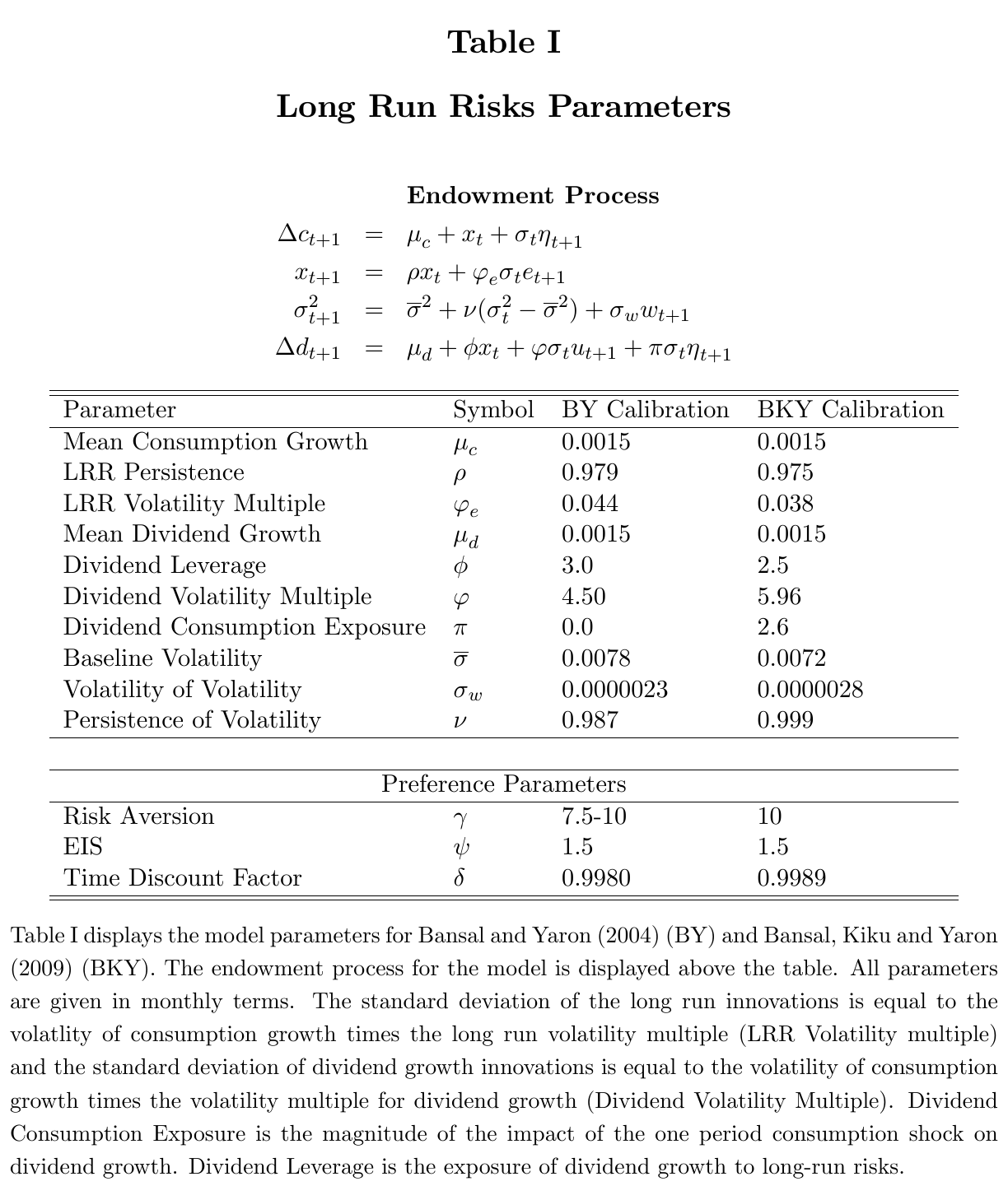
Table I looks like two calibrations of the same model, and line by line it nearly is. Expected-growth persistence is 0.979 against 0.975, half-lives of 33 and 27 months. Volatility shocks have “similar standard deviations”. The difference is one number: $\nu$ is 0.987 in by and 0.999 in bky, which takes the half-life of a volatility shock from “slightly over four years” to 58 years. That one number changes what the model is about. Shut volatility off and by’s equity premium barely moves (5.4% with constant volatility, 5.5% with it), and its $p-d$ volatility is 0.18 either way. In bky the same switch takes the premium from 3.8% to 6.6% and the volatility of $p-d$ from 0.13 to 0.18 (text, pp. 13–14). by is a growth-risk model with some volatility in it. bky is a model in which volatility risk is primary, with growth still doing much of the work.

A 58-year half-life has a side effect the authors note with some restraint. A variance that persistent, hit by normal shocks, wanders below zero: in bky it goes negative in 1.3% of months, and over half of 79-year simulated paths go negative at some point, against under 0.2% of paths in by. The simulation censors it at a small positive number and carries on. It is not the paper’s main complaint, but it is a sign of how close to a unit root the recalibration had to push to get where it needed to go.

The method: simulate the model, run the data’s regressions on it

There is no estimation here. The authors take each calibration as published and ask whether us history looks like a draw from it. They simulate monthly, with a ten-year burn-in, and aggregate exactly the way the data are built: consumption and dividend levels summed over the quarter or year before taking growth, log returns summed, and $p - d$ as the year-end price over the previous year’s dividends. They draw 100,000 samples of the data’s length (948 months for annual 1930–2008, 741 for quarterly 1947.2–2008.4), run the same regression on each, and report the model median and the data statistic’s percentile in the model distribution. Below 0.05 or above 0.95 is bold, which the table notes call “a 5 percent one-sided test or a 10 percent two-sided test”. The data are the usual ones: bea real nondurables and services per capita, crsp value-weighted returns and dividends, and an ex-ante real rate built by projecting the realised bill return on the nominal yield and lagged inflation. The annual sample is identical to bky’s.

This is the right test for a calibrated model with persistent states. The question isn’t whether the parameters are right. It’s whether this particular 79-year history is something the model would plausibly produce.

The evidence: what the price–dividend ratio knows

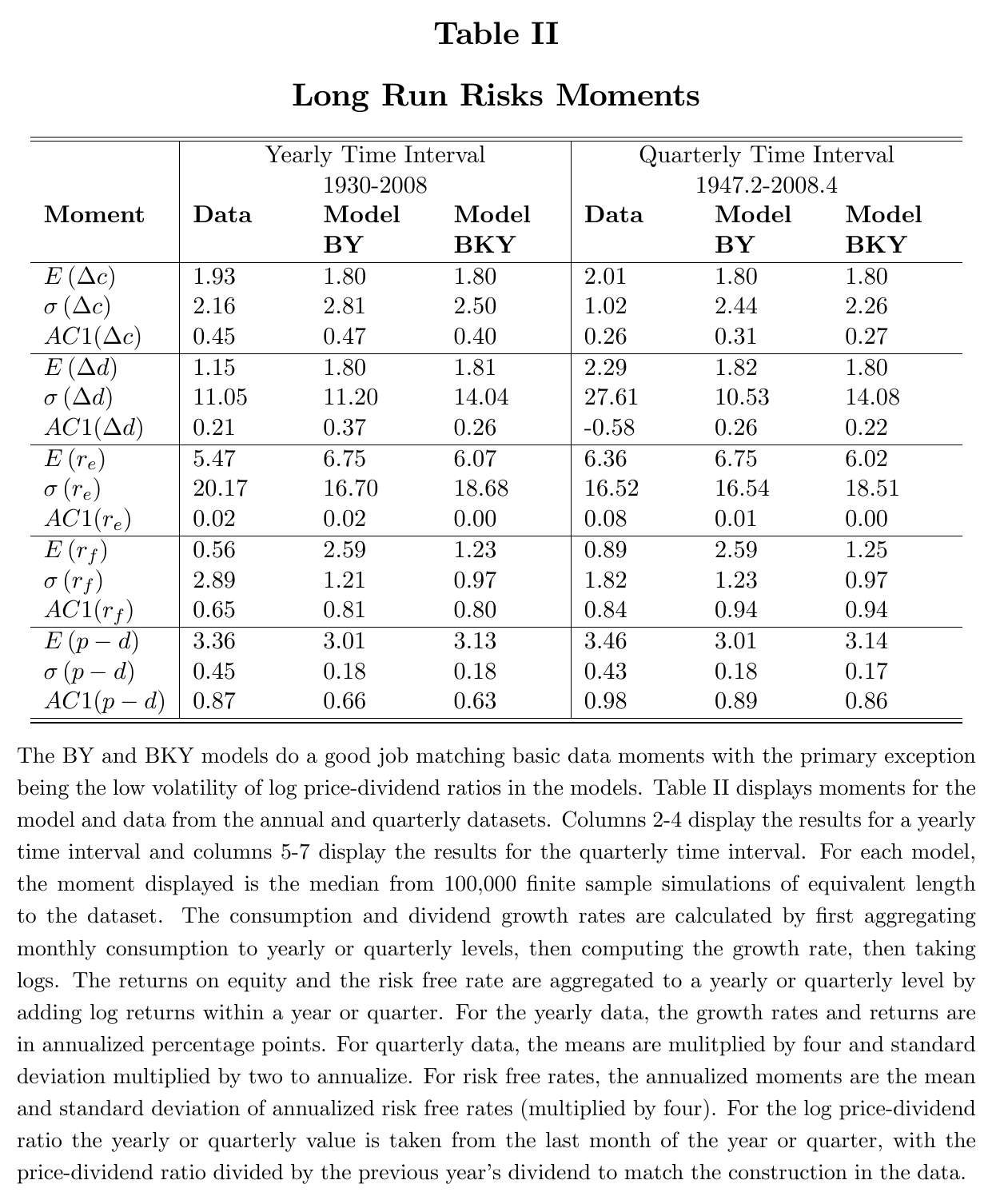
Table II is the polite part. Means, volatilities and first autocorrelations of consumption growth, dividend growth and excess returns are matched reasonably in annual data. But the price–dividend ratio has a standard deviation of 0.45 in the data and 0.18 in both calibrations (0.36 if you stop in 1998, as by did, “still somewhat higher”), and it is also more persistent, with an annual autocorrelation of 0.87 against 0.66 and 0.63. The real rate’s standard deviation is 2.89% against 1.21% and 0.97%. And postwar quarterly consumption growth has an annualised volatility of 1.02%, against 2.44% and 2.26% in the models, which the authors call “a more serious difficulty”.

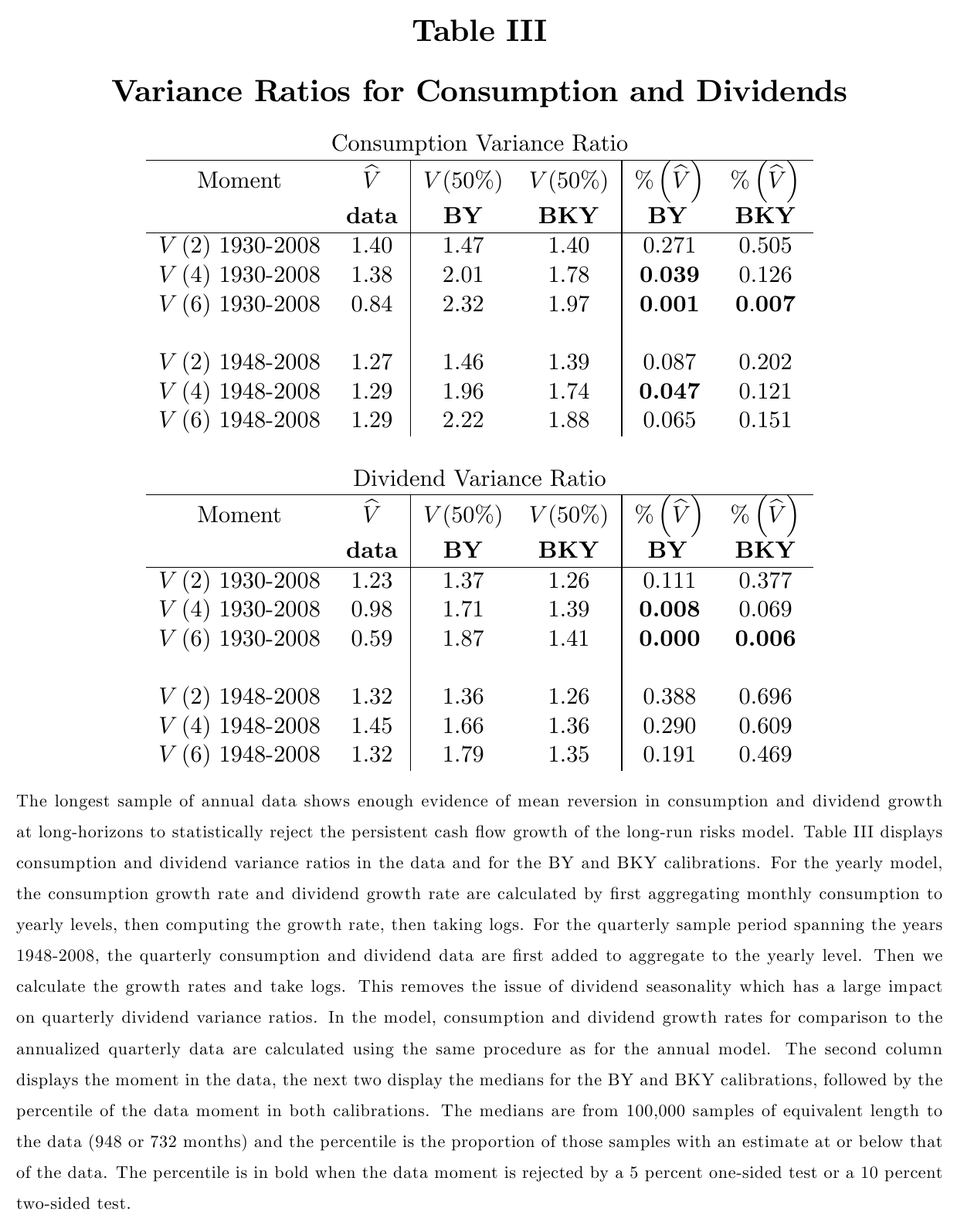
Persistence first. A variance ratio $V(K)$ compares the variance of $K$-year growth to $K$ times the one-year variance, so a slow-moving $x_t$ pushes it above one. In 1930–2008 the six-year ratio is 0.84 for consumption and 0.59 for dividends. The model medians are 2.32 (by) and 1.97 (bky) for consumption and 1.87 and 1.41 for dividends, and the data sit at percentiles of 0.001, 0.007, 0.000 and 0.006. Fewer than 1% of simulated samples look this mean-reverting. The two-year ratios of 1.2 to 1.4 are about what time-averaging a random walk gives you, which is 1.25 (Working 1960). Postwar the picture is softer: six-year ratios of 1.29 for consumption and 1.32 for dividends, and neither calibration is rejected at that horizon (though by’s postwar four-year consumption ratio, at percentile 0.047, is).

The model has a ready answer to this, and it’s the answer that makes the rest of the paper possible. Of course univariate statistics can’t find $x_t$; it is buried under transitory noise. But then investors must see it some other way, and prices must carry it.

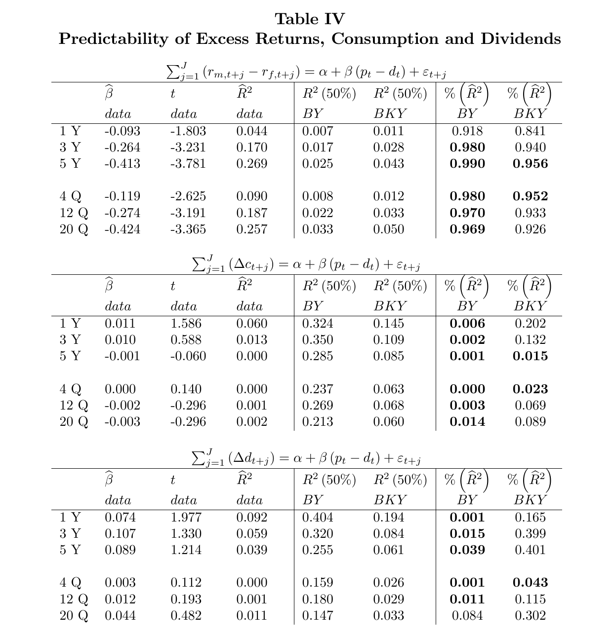
Table IV is where that fails. Regress future consumption growth on $p - d$ in 1930–2008. The five-year $R^2$ is 0.000. by’s median is 0.285 (percentile 0.001) and bky’s is 0.085 (percentile 0.015). At one year the data give 0.060 against 0.324 for by (rejected) and 0.145 for bky (not rejected), and in quarterly postwar data the four-quarter $R^2$ is 0.000 against 0.237 and 0.063, rejecting both. Dividends tell a gentler version of the same story: annual $R^2$ of 0.092, 0.059 and 0.039 at one, three and five years, against by medians of 0.404, 0.320 and 0.255, all rejected, and bky medians of 0.194, 0.084 and 0.061, none rejected.

Meanwhile $p - d$ forecasts excess returns very nicely, with $R^2$ of 0.044, 0.170 and 0.269 at one, three and five years. by’s medians are 0.007, 0.017 and 0.025, and bky’s are 0.011, 0.028 and 0.043. Stambaugh (1999) bias fattens the right tail of the model’s $R^2$ distribution, so the authors only claim rejection beyond one year in annual data: percentiles 0.980 and 0.990 for by and 0.940 and 0.956 for bky at three and five years (the quarterly four-quarter column, at 0.980 and 0.952, rejects both as well). The authors’ summary of by is that these patterns are “the reverse of the predictions”. In the model, $p - d$ moves because expected cash flows move. In the data, it moves because expected returns move.

Two more checks close the doors. In the model, $p - d$ is as correlated with past consumption growth as with future growth, because $x_t$ is. In the data, the lead–lag correlations are much lower and shifted towards the past, so prices respond to consumption that has already happened more than they anticipate consumption to come (the paper’s Figures 1 and 2). That pattern is habit-like, the authors note, though Campbell and Cochrane (1999) also make the price–consumption link too strong.

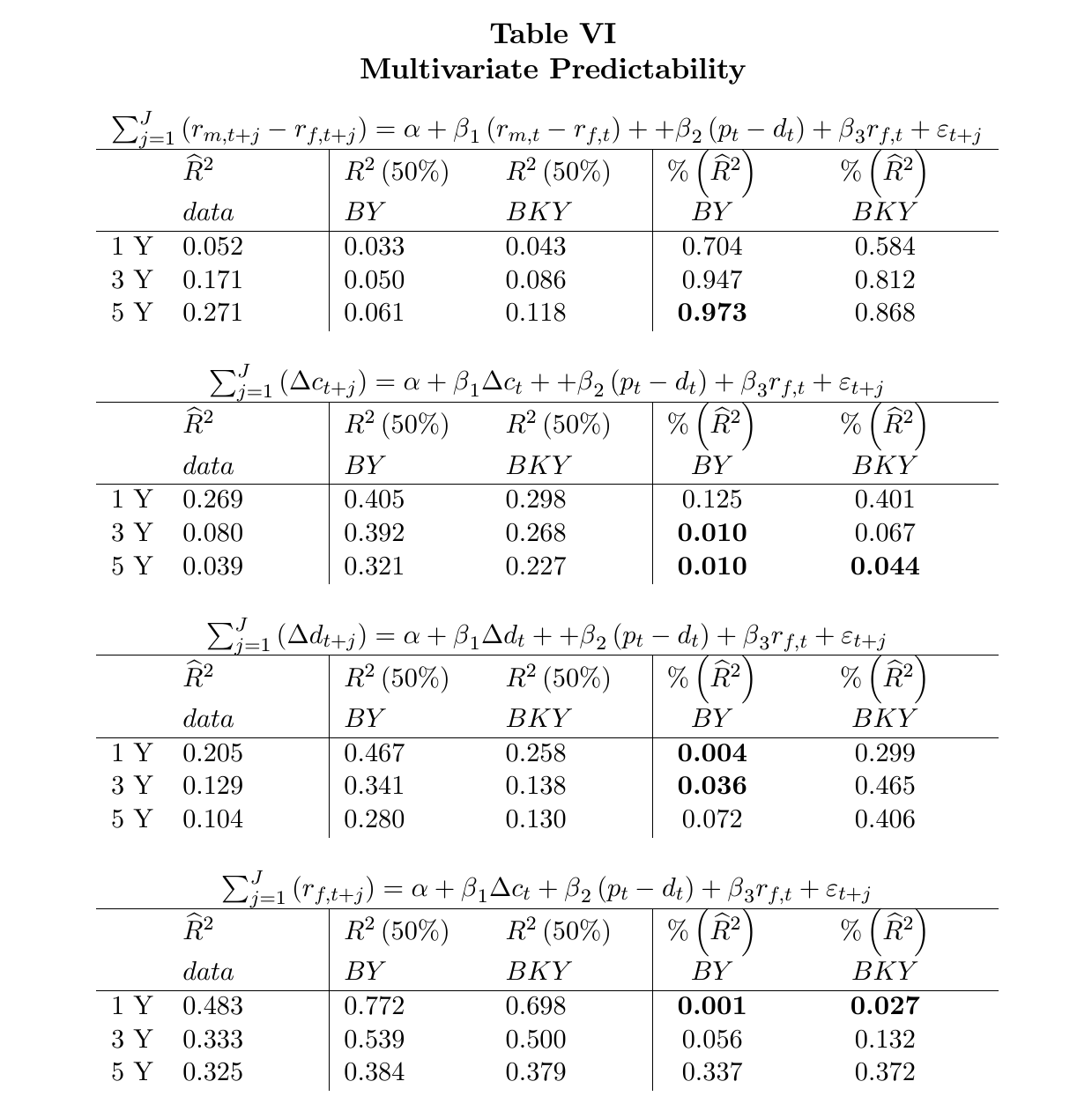
The second check is bky’s own evidence. bky find cash-flow predictability using a var(1) in lagged growth, $p-d$ and the real rate, which implies five-year $R^2$ of 22% for consumption and 28% for dividends. Beeler and Campbell keep the information set and drop the var: the same predictors in direct long-horizon regressions give 0.039 for consumption and 0.104 for dividends at five years (Table VI). The gap, they argue, is misspecification. Time-averaged consumption looks like an ma(1), and a var(1) fitted to it extrapolates short-run momentum into long-run predictability. What dividend predictability survives comes from lagged dividend growth with a negative sign, which is mean reversion and so, in the authors’ words, “evidence against the long-run risks model rather than evidence for it”.

The one surprising thing

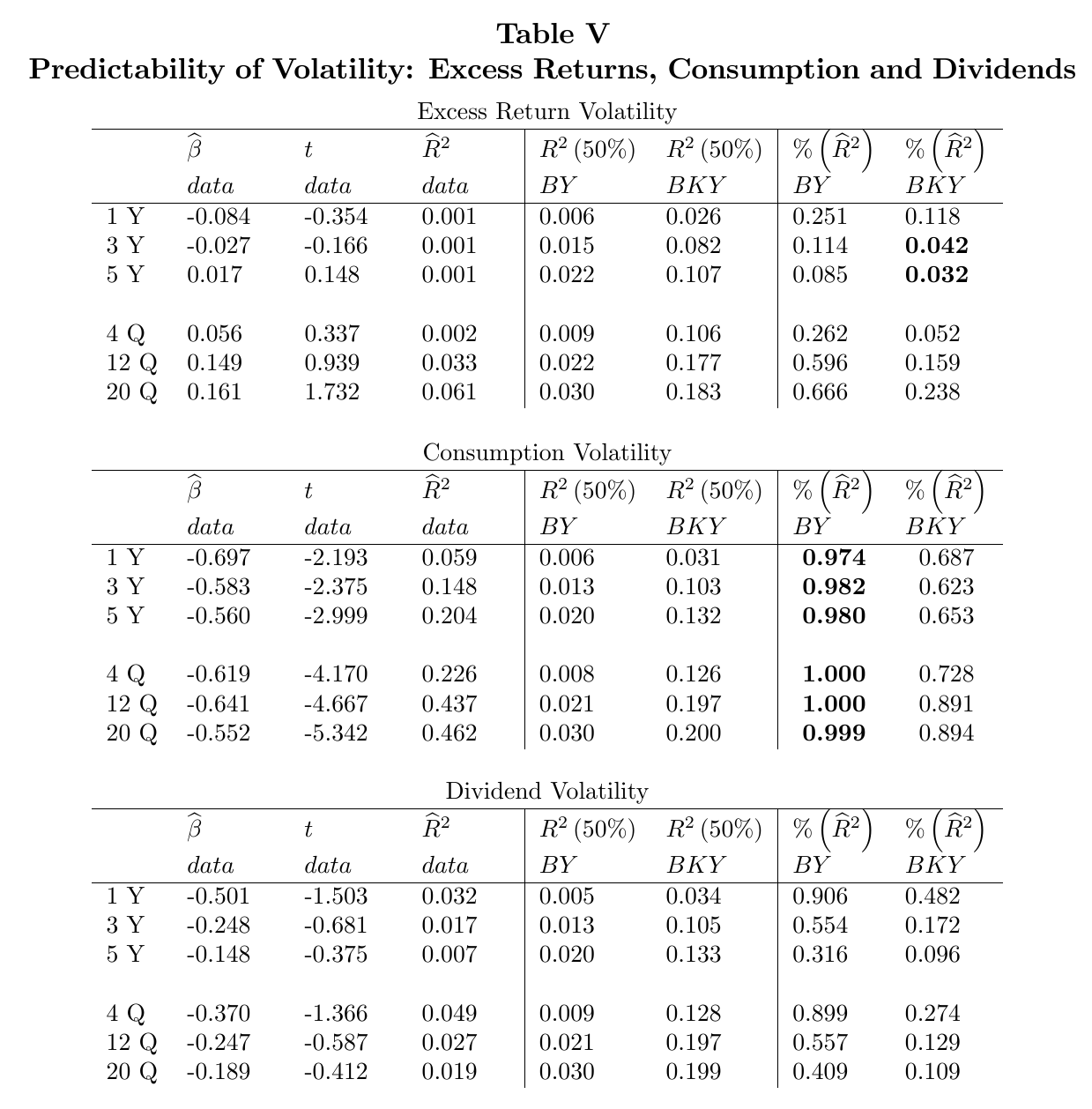
bky’s recalibration is a reasonable response to all this. If $p-d$ forecasts growth too well under by, turn the dial so that $p-d$ is largely about $\sigma_t^2$, and its forecasts of growth shrink. And this move hits a real fact that by misses. Measure realised volatility as the sum of absolute ar(1) residuals over $K$ periods, regress its log on $p - d$, and in the data the ratio forecasts consumption volatility strongly and with the right negative sign: five-year $\beta = -0.560$ with $R^2$ of 0.204 annually, and an $R^2$ of 0.462 at 20 quarters postwar. by’s medians are 0.020 and 0.030 (percentiles 0.980 and 0.999), so by is rejected. bky’s are 0.132 and 0.200, comfortably inside the distribution. On consumption volatility, bky wins.

Now apply eq. 3 again. In bky, $\sigma_t$ scales every growth and cash-flow shock in the economy, including the ones that drive stock returns, and $p-d$ is in large part a reading of $\sigma_t^2$. So $p-d$ should forecast the volatility of stock returns as well. bky’s median five-year $R^2$ for return volatility is 0.107 annually and 0.183 quarterly. The data give 0.001 and 0.061, and the quarterly coefficient has the opposite sign to the model’s. The annual misses reject at three and five years (percentiles 0.042 and 0.032), and the one-year quarterly one is “almost significant” (0.052), though the five-year quarterly miss is not (0.238). The authors put the puzzle plainly: “why don’t they forecast the future volatility of the stock market itself?”

So stock prices know something about future consumption risk and almost nothing about their own future risk. by passes the return-volatility test, but only because its $p - d$ knows almost nothing about volatility of any kind, which is exactly why it fails on consumption volatility. There is one signal and two promises, and turning the dial to keep one promise breaks the other. The authors leave it as an open problem, and it is a good one: a model where valuations track macro risk but not market risk needs something to come between the two.

The other bills: real bonds and the eis

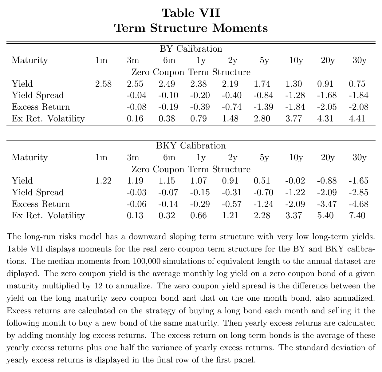
Real bonds are a hedge in this model. Bad growth news lowers real rates and raises bond prices, and so does a volatility shock through precautionary saving, both in states where marginal utility is high. So long real bonds pay off when you need it, term premia are negative, and the real curve slopes down, more so the more persistent volatility is. In Table VII the by 30-year real yield sits 1.84 points below the short rate, and about one point below the five-year yield. Under bky the 30-year real yield averages −1.65%, the spread to the short rate is −2.85 points, and the 30-year bond’s average excess return is −4.68%. Persistent volatility makes the far future so uncertain that the safe long rate collapses. The table has no data column, because there are fewer than fifteen years of tips, but the authors note that the tips curve has never had a quantitatively significant negative slope, and that long tips yields have been always positive and usually above 2% (Campbell, Shiller and Viceira 2009). Worse, the late 1990s and 2000s had high valuations, which in the model signal high expected growth or low volatility and so an inverted real curve, which is the opposite of what was seen.

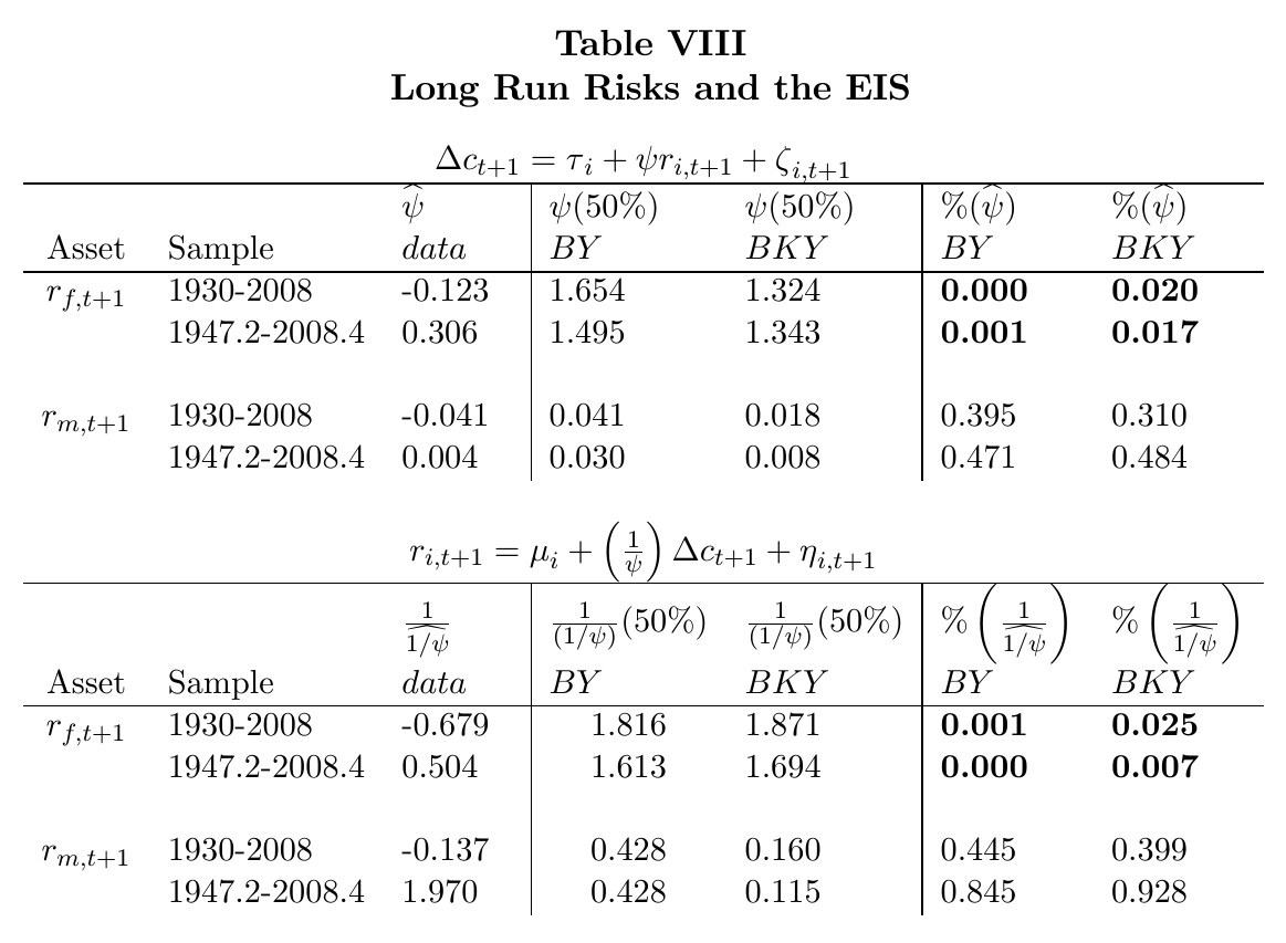
The last bill is the eis. The model needs $\psi > 1$; with $\psi = 0.5$, by’s premium shrinks and its risk-free rate rises, and under bky the consumption claim’s price becomes infinite (pp. 26–27). The test is the Hall (1988) regression:

This is eq. 16 in the paper: $\psi$ is the eis, $r_{i,t+1}$ is the real bill rate or the stock return, $\zeta_{i,t+1}$ is the Euler-equation error, and the equation is estimated by 2SLS with instruments lagged twice. With the bill rate, the data give $\hat\psi = -0.123$ annually and 0.306 quarterly. The model’s own simulated estimates have medians of 1.654 and 1.495 under by and 1.324 and 1.343 under bky, with percentiles of 0.020 or below in every case. With the stock return as the asset, the model’s own iv estimates are biased towards zero and noisy, presumably weak instruments, and nothing can be rejected.

Bansal and Yaron’s defence was that heteroskedastic consumption biases these regressions down. The authors call it “correct in principle” and then measure it: under by there’s no downward bias with the bill rate, and under bky there is some bias, but the median estimates with the bill rate still stay above 1.3. The authors’ conclusion leaves a contradiction for someone else. Consumption that ignores predictable movements in real rates says the eis is low. Stock prices that fall when consumption volatility rises say it is high.

Objections the paper sees coming

The sample. bky argue that the long annual sample should be primary and that the Depression years carry important information. The authors keep the annual sample (it is bky’s) and add postwar data as an outlier check. Then they turn the Depression around: consumption fell 18% over 1930–33, and four-year declines that large occur in 6.9% (by) and 6.6% (bky) of simulated samples, but the fall followed by a 19% rise over 1934–37 occurs in only 0.1% and 0.3%. A rare-disaster model (Barro 2006) fits that episode much better. (My own reading: the cut works both ways, since postwar data reject less on persistence but miss worse on consumption volatility and reject at short quarterly horizons.)

Only one calibration. bky evaluate only their high-persistence calibration. The authors evaluate both because much of the literature still uses by-like volatility persistence, and because the contrast shows how sensitive the model is to one parameter.

Method. by’s original predictability exercise gave “qualitatively similar but quantitatively less extreme results” with a numerical solution since abandoned in the literature; the analytical loglinear solution here is what bky themselves use. Time aggregation is replicated in the model, consumption timing follows by’s end-of-period convention (which favours lagged financial predictors; beginning-of-period results are similar), and a Tornqvist-index version of consumption growth gives similar results.

Better consumption data. Disaggregated or stockholder consumption gives higher eis estimates, but the long-run risk model is calibrated to aggregate consumption, so a limited-participation version is “a different model that remains to be explored”.

What stays open, by the authors’ account, is other parameters or extensions (habits, disasters, cointegration of consumption and dividends) estimated by gmm against exactly these predictive moments, which they concede is hard with this many parameters, this little data and states this persistent.

A note on the reply (outside the paper)

The Critical Finance Review printed a reply by Bansal, Kiku and Yaron (2012) in the same issue. This note doesn’t cover it. What is said about bky above is only what the October 2011 version says about their then-unpublished paper: its sample argument, its var evidence, and its focus on the high-$\nu$ calibration.

Why this matters for growth and asset pricing: identification by prices

For a reading list on growth and asset pricing, this is the paper that sets the identification problem. Long-run risk puts its key state where the econometrician can’t see it, and it can only do that because prices are supposed to see it instead. That makes prices the identifying instrument, and Beeler and Campbell show what the instrument says: valuations carry information about discount rates and about macro volatility, and almost none about long-run growth. Anyone who wants to give $x_t$ a physical source, like R&D in Kung and Schmid (2015) or Franceschini (2026), inherits both halves of the test. The source has to forecast growth, and markets have to price it, without valuations forecasting cash flows any better than they actually do. Which is why that literature measures growth risk in quantities and checks whether returns load on it, rather than reading it off $p - d$. That is a sensible design, and it is also a quiet concession that the price–dividend ratio, the model’s own window onto long-run growth, turned out to be looking mostly at something else.

References