Risks for the Long Run: A Potential Resolution of Asset Pricing Puzzles

Ravi Bansal and Amir Yaron, The Journal of Finance 59 (4), 2004, pp. 1481–1509. Published version; no recorded talk.

Bansal and Yaron’s paper is the founding document of long-run risk, and its trick fits in one sentence: put a drift in consumption growth that is too small to see and too persistent to ignore, and give the investor preferences that care about the difference. The problem it attacks is old. Mehra and Prescott (1985) showed that consumption is too smooth to justify a 6% equity premium unless risk aversion is absurd, Weil (1989) showed that pushing risk aversion up under the usual preferences then sends the risk-free rate somewhere silly, and stock prices move far more than any news about dividends seems to warrant. The standard escape routes all change the investor: habits, heterogeneity, behavioural stories. Bansal and Yaron keep a representative agent with Epstein–Zin (1989) preferences and change the cash flows instead, but only by an amount the consumption data cannot reject. That is either very elegant or a little suspicious, depending on how you feel about variables you can’t observe, and the paper is unusually candid that it is both.

The mechanism: a drift too small to see, priced as if it were huge

The cash-flow side is four lines. Expected consumption growth has a component $x_t$ that wanders slowly around its mean $\mu$, and every cash-flow shock is scaled by a common volatility $\sigma_t$ that also wanders slowly:

This is eq. 8 in the paper: $g$ and $g_d$ are log consumption and dividend growth, $x_t$ the persistent expected-growth component with persistence $\rho$, $\sigma_t^2$ the conditional variance (“economic uncertainty”) reverting to $\sigma^2$ at rate $\nu_1$, $\phi$ the dividends’ leverage on $x_t$, and $\varphi_e$, $\varphi_d$ the shock scales.

The calibration is monthly, with $\rho = 0.979$, $\nu_1 = 0.987$, $\phi = 3$ and $\varphi_e = 0.044$. That last number is the whole game. The paper reports that $x_t$ accounts for only 4.4% of the variance of monthly consumption growth. You would not find it by staring at consumption, and the paper does not claim you would.

Now the preferences. With Epstein–Zin utility the log pricing kernel is $m_{t+1} = \theta\log\delta - (\theta/\psi)g_{t+1} + (\theta - 1)r_{a,t+1}$, where $\psi$ is the ies, $\gamma$ is risk aversion, $\theta = (1-\gamma)/(1-1/\psi)$, and $r_a$ is the return on a claim to aggregate consumption (eq. 3 in the paper). Under power utility $\theta = 1$, the last term vanishes, and the kernel only cares about this month’s consumption growth. At the paper’s $\gamma = 10$ and $\psi = 1.5$, $\theta$ is about −27 (my arithmetic), and the kernel cares a great deal about the return on wealth, which is to say about anything that moves the value of all future consumption. News about $x_t$ and $\sigma_t^2$ moves it a lot, and that is where the premium comes from.

How much it moves depends on the valuation loadings. Log-linearise returns à la Campbell and Shiller (1988) and the price–consumption ratio is affine in the states, $z_t = A_0 + A_1 x_t + A_2\sigma_t^2$, with

These are eqs. 5 and 9 in the paper: $A_1$ and $A_{1,m}$ are the responses of the consumption claim’s and the market’s log valuation ratios to $x_t$, $A_2$ the response to $\sigma_t^2$, and $\kappa_1, \kappa_{1,m} \approx 0.997$ the Campbell–Shiller linearisation constants.

Read the denominators first. With $\kappa_1 \approx 0.997$ and $\rho = 0.979$, $1 - \kappa_1\rho$ is about 0.024, so a unit of expected-growth news is multiplied by roughly 40 on its way into prices. That is what persistence buys: a shock to the growth rate that lasts for years is a shock to the level of everything, and the price capitalises all of it at once. Then read the numerators. $A_1 > 0$ requires $\psi > 1$: good news about growth raises prices only if the substitution effect beats the wealth effect. Under power utility with $\gamma > 1$ you are stuck with $\psi < 1$, and good growth news lowers prices, because the risk-free rate rises enough that discounting wins. That is a strange world in which booms are bad for the stock market, and the paper is right to treat escaping it as a requirement rather than a taste. Dividends lever up the effect, since $\phi = 3$ makes $A_{1,m}$ larger than $A_1$. And because $\theta < 0$, $A_2$ is negative: more uncertainty, lower valuations, and the paper says plainly that “an ies larger than 1 is critical” for that sign.

The kernel’s innovation then has three pieces:

This is eq. 10 in the paper: $\lambda_{m,\eta} = -\gamma$, $\lambda_{m,e} = (1-\theta)\kappa_1 A_1\varphi_e$ and $\lambda_{m,w}$ are the prices of short-run consumption risk, long-run growth risk and volatility risk, and both $\lambda_{m,e}$ and $\lambda_{m,w}$ are zero under power utility ($\theta = 1$).

A note on signs, since this trips people up. In the printed convention $\lambda_{m,w}$ is itself negative ($\theta < 0$ and $A_2 < 0$), and the equation subtracts it, so a positive volatility shock raises the kernel. The market’s exposure to $w$ is also negative, so the product that enters the premium is positive: the market falls exactly when marginal utility jumps, which is what “volatility risk carries a positive premium” means. The resulting equity premium (eq. 11 in the paper) is $\beta_{m,e}\lambda_{m,e}\sigma_t^2 + \beta_{m,w}\lambda_{m,w}\sigma_w^2 - 0.5\,\mathrm{var}_t(r_m)$, two priced risks plus a Jensen term. The first term moves with $\sigma_t^2$, so the premium and the Sharpe ratio vary over time, and that is where return predictability comes from.

Notice what is not priced at a premium. The dividend-specific shock $u$ is large and earns nothing. The short-run consumption shock $\eta$ earns only the usual $\gamma$ times a small covariance. The money is all in two small, slow things.

The evidence: does the drift survive contact with the data?

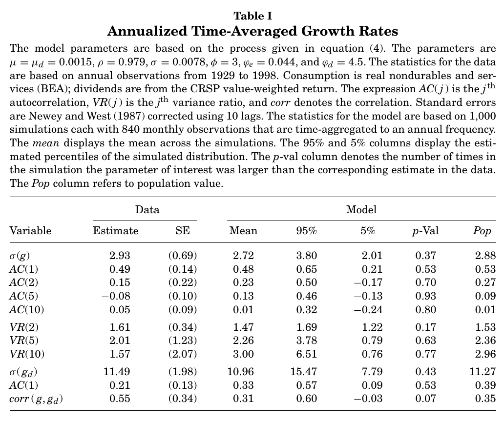
The data are annual us real per-capita nondurables and services consumption, plus crsp value-weighted dividends and returns, 1929–1998. Table I is the defence of the drift. The authors simulate 1,000 samples of 840 months from the persistent model, aggregate to annual, and ask whether the data look like a draw. They mostly do. Consumption volatility is 2.93% in the data against 2.72% in the model, and first-order autocorrelation is 0.49 against 0.48. The weak spots are at long lags. The data’s ac(5) is −0.08 against the model’s 0.13, which the authors call “slightly above the two standard error range”, and the data’s variance ratios rise and then turn down at about seven years while the model’s keep climbing (vr(10) of 1.57 against 3.00, inside a very wide band). The model’s consumption–dividend correlation, 0.31 against 0.55, is low, which they call conservative. The honest summary is that the annual data are compatible with this process, not that they reveal it.

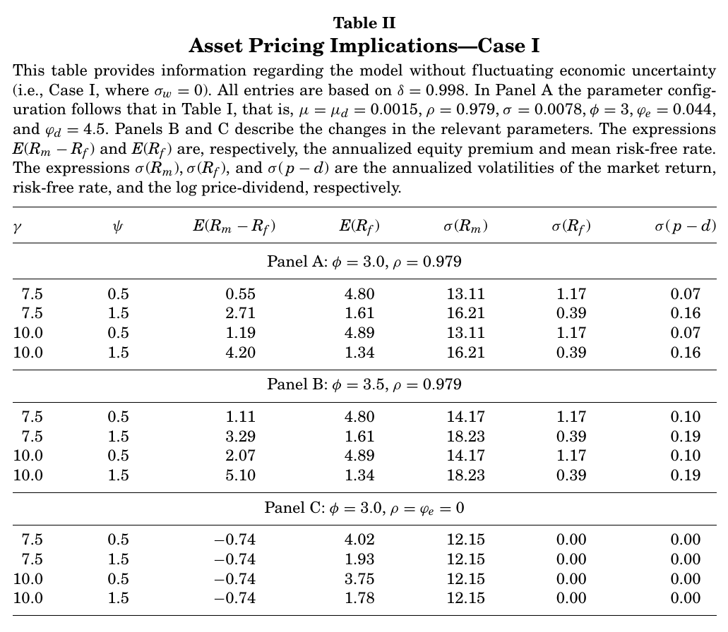
Table II turns on only the growth channel, with volatility held constant. At $\gamma = 10$ and $\psi = 1.5$ the equity premium is 4.20% with a risk-free rate of 1.34%. Drop the ies to 0.5 and the premium falls to 1.19% while the risk-free rate jumps to 4.89%: this is the risk-free-rate puzzle reappearing on cue. Panel C sets $\rho = \varphi_e = 0$, making growth i.i.d., and the premium becomes −0.74% for every preference setting. That number is not a negative risk premium in any interesting sense. With dividend and consumption shocks independent, the covariance term is zero and all that is left is $-0.5\,\mathrm{var}(r_m)$, the Jensen term on a log-return premium. In other words, zero. The authors add that a 0.25 monthly consumption–dividend correlation would lift it to 0.08% a year, which is Mehra and Prescott’s answer again.

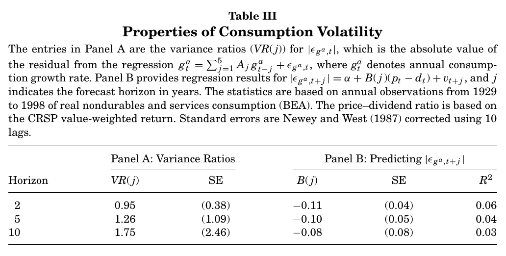
Table III is the case for time-varying volatility. If consumption residuals had constant variance, the variance ratios of their absolute values would be flat across horizons. They rise, from 0.95 at two years to 1.75 at ten, though with standard errors (0.38, 1.09, 2.46) as large as the estimates. The price–dividend ratio predicts lower future realised volatility, with a slope of −0.11 (s.e. 0.04) at two years that fades to insignificance by ten. That is suggestive, and the paper defers the robustness work to Bansal, Khatchatrian, and Yaron (2002).

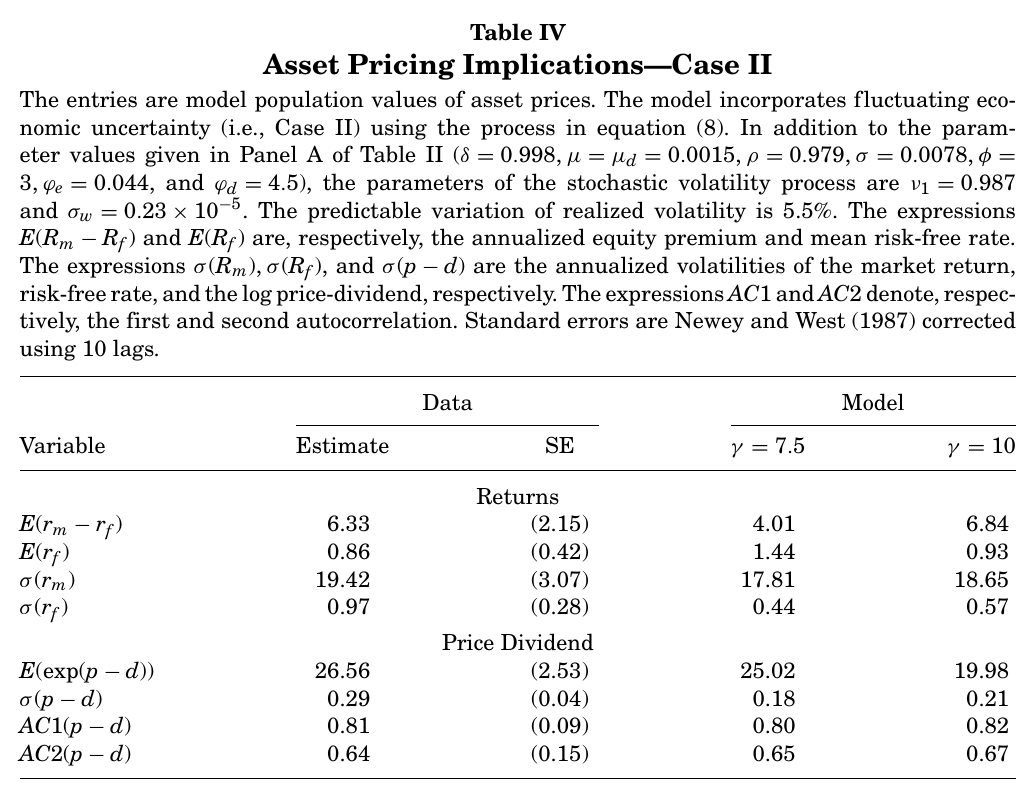
Table IV is the headline. Turn volatility on, keep $\psi = 1.5$ and $\gamma = 10$, and the model delivers an equity premium of 6.84% against 6.33% (s.e. 2.15) in the data, a risk-free rate of 0.93% against 0.86%, and market volatility of 18.65% against 19.42%. Relative to Table II the premium rises by about 2.5 points, which the paper attributes to the volatility-risk term in eq. 11 (strictly, it is a comparison of two equilibria, not a decomposition of one). The price–dividend ratio’s persistence is right on: 0.82 against 0.81. The text then says the model “essentially duplicates” the volatility and persistence of the price–dividend ratio. On volatility it does not. The model’s $\sigma(p-d)$ is 0.21 against 0.29 with a standard error of 0.04, two standard errors short, and the mean price–dividend level is about 20 against 26.6. Risk-free volatility is also low, 0.57 against 0.97. It is a very good fit for a model with no habit and no heterogeneity, and it is not a duplicate.

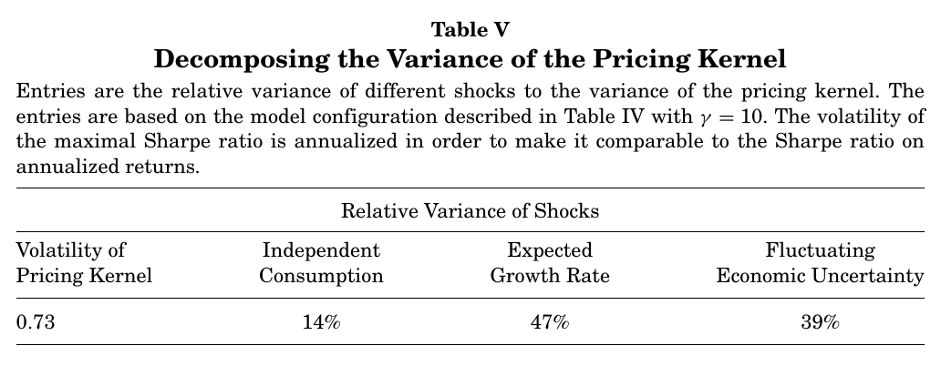
Table V asks what the kernel is made of. The maximal annualised Sharpe ratio is 0.73, well above the market’s 0.33. Of the kernel’s variance, 14% comes from the short-run consumption shock $\eta$, 47% from expected-growth news $e$, and 39% from volatility news $w$. So growth news is the largest single source, not a majority, and volatility news is close behind. The comparison the paper offers is that with i.i.d. growth and constant volatility the maximal Sharpe ratio would be $\gamma\sigma$, or 0.27 annualised. That is not the full model with $x_t$ switched off, since volatility news would still be there; the paper credits “the Epstein and Zin preferences and the departure from i.i.d. growth rates” jointly, and that is the right way to read it.

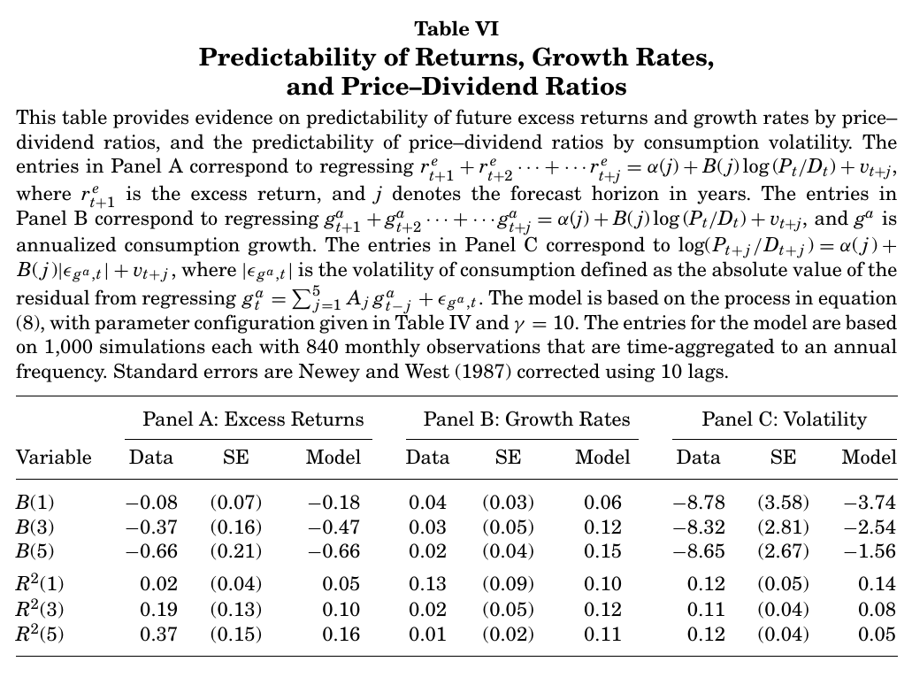
Table VI is predictability, and it is where the paper is weakest, though you have to read the numbers rather than the prose to see it. Panel A regresses future excess returns on the log price–dividend ratio. The slopes line up well (−0.66 at five years in both data and model), but the model’s five-year R² is 0.16 against 0.37 in the data. Panel B regresses future consumption growth on the same ratio. The authors describe slopes and R² as “quite low both in the data and the model”. At one year that is fair. At five years the model’s slope is 0.15 with an R² of 0.11, while the data’s are 0.02 and 0.01. The model predicts consumption growth from valuations much better than the world does, which is exactly what you would expect if half of the variation in valuations is cash-flow news, and the paper’s own Cochrane-style decomposition says it is (52% returns, 54% dividend growth in population, against 108% and −6% in the data with huge standard errors). Panel C gets the sign of volatility predicting valuations right, at roughly a third to a fifth of the data’s magnitude.

The one surprising thing

The surprising thing is that the same consumption data support two opposite pricing worlds, and the paper says so in as many words: the persistent and i.i.d. processes are “difficult to distinguish”, but their “asset pricing implications are vastly different”. Hold preferences fixed at $\gamma = 10$, $\psi = 1.5$. With a component that explains 4.4% of monthly consumption growth, the equity premium is 4.20%. Without it, zero minus a Jensen term. Nothing in Table I could tell you which world you are in; the claim that finite samples cannot reject i.i.d. growth is borrowed from Shephard and Harvey (1990) rather than simulated here, but the bands in Table I make the converse plain. So the stock market is doing the econometrics. The paper is, in effect, using asset prices as the instrument that detects a component of consumption the consumption data cannot see, and then using that component to explain asset prices. This is not circular, exactly, because the calibration also has to fit consumption moments, the risk-free rate and the predictability tables. But it means the equity premium is the main evidence for $x_t$, and $x_t$ is the main explanation for the equity premium, and you should hold that thought for the pushback section.

The runner-up is quieter and arguably more useful. Run Hall’s (1988) regression of consumption growth on the risk-free rate in data simulated from the model, where the true ies is 1.5, and you estimate 0.62. Time-varying volatility moves the risk-free rate for precautionary reasons that have nothing to do with intertemporal substitution, and that biases the slope down. The low ies estimates that make $\psi > 1$ look reckless may themselves be artefacts of ignoring volatility.

Objections the paper sees coming

There is no discussant, but the paper argues with several imaginary ones, and the answers are worth having in one place.

The first is that consumption growth is close to i.i.d. and $\rho = 0.979$ is invisible. The answer is Table I plus Shephard and Harvey, and the post-war first-order autocorrelations (0.38 for 1951–1999, 0.44 for 1961–1999) both fall inside the model’s simulated band. They also explain why $\rho$ is below one rather than the unit root of Barsky and DeLong (1993): stationarity.

The second is that an ies above one contradicts Hall (1988) and Campbell (1999). The answer has three parts. Other estimates exceed one (Hansen and Singleton, Attanasio and Weber, Vissing-Jorgensen, Guvenen). The Hall regression is biased down in this very model, 1.5 to 0.62. And with $\psi < 1$ and moderate risk aversion, Table II shows the risk-free rate becoming high and volatile.

The third is why this works when earlier Epstein–Zin attempts did not. Weil (1989) used i.i.d. growth, so had no long-run risk to price. Kandel and Stambaugh (1991) had, at this paper’s preference parameters, too little persistence and, in the paper’s words, “primarily focus on the case in which the ies is close to zero”.

The fourth is that predictability is fragile and valuation ratios are mostly discount-rate news. Here the authors concede more than they rebut. They cite the sample-sensitivity literature themselves, allow that cash dividends may mismeasure total payouts, point to the wide standard errors on the data’s decomposition, and note that in small samples the model’s returns share rises to about 70%.

The rest are concessions stated as such. The variance process can go negative, and in about 5% of realisations negative draws are replaced by a tiny number, which the authors call “primarily a technical issue”. The shocks are assumed independent, which they call conservative, since a 0.25 correlation between dividend and growth shocks would push the premium from 4.20% to about 5.2%. Cointegration between consumption and dividends is ignored and left for future work. And the model can only produce a positive relation between expected returns and market volatility, so it cannot match the negative relation some studies find; they conjecture that fixing it “will require significant changes”, perhaps along the lines of Whitelaw’s (2000) regime-switching power-utility model, and leave it there.

Later pushback (outside the paper)

The following is from the subsequent literature, not from this paper. Beeler and Campbell (2012) pressed precisely on Table VI Panel B: the calibration implies that valuations forecast consumption and dividend growth far better than they do, and returns less well. Bansal, Kiku and Yaron (2012) responded in the same issue with a recalibration built on much more persistent volatility. Epstein, Farhi and Strzalecki (2014) asked what the preferences imply about the timing of resolution of uncertainty, and found that long-run-risk calibrations have agents willing to give up an implausibly large share of consumption just to learn the future early. The literature that tries to give $x_t$ an observable source, such as R&D in Franceschini (2026), is in part a response to the first of these.

All of which leaves the paper where its title, with its careful “potential”, put it. It shows that a tiny, slow drift in growth plus a recursive investor can carry most of the classic puzzles at once, and it is honest that the drift is nearly invisible in the quantity it drifts. The equity premium, it turns out, may be the price of the one thing about consumption we cannot measure, which is a bold claim and also, if you think about it, exactly what you would expect a risk premium to be.

References