Banking, Trade, and the Making of a Dominant Currency

Gita Gopinath and Jeremy C. Stein, both of Harvard’s economics department (Gopinath by then also the imf’s chief economist), “Banking, Trade, and the Making of a Dominant Currency”, published in the Quarterly Journal of Economics 136(2), May 2021, pp. 783–830, advance access October 2020. No talk recording of this paper exists, so this is a read of the document alone. Digested from the published version, which supersedes nber Working Paper 24485 of 2018; the model was reformulated in between, and where the two differ the published propositions are what is described here.

A deposit is a promise denominated in something

You are a household in Turkey. You hold a buffer of bank deposits because you are going to buy imported things with them over the next few periods, and about 60% of the imports you buy are invoiced in dollars — this is Gopinath’s (2015) number, and the companion fact is that only 6% of Turkey’s imports actually come from the United States. Now ask which deposit is safe for you. A lira deposit is default-free. A dollar deposit is default-free. But only one of them buys a known quantity of the goods you are actually going to buy, because the prices of those goods are sticky in dollars. The paper’s opening observation is that “a financial claim is only meaningfully ‘safe’ if it can be used to buy a known quantity of some specific goods at a future date, and this necessarily forces one to ask about how the goods will be priced.”

That sentence is the whole paper, and it has a consequence that runs backwards through the plumbing. If invoicing decides what “safe” means, then the volume of dollar-invoiced trade is a demand curve for dollar safe assets. The us Treasury supplies some of that. The rest has to be manufactured, and the manufacturers are banks in emerging markets, whose borrowers mostly earn local currency. A bank that promises you a dollar tomorrow needs assets that will be worth a dollar tomorrow in every state of the world, including the state where the local currency has collapsed. Peso revenue is a bad input for dollar promises. It works, but you need a lot more of it.

So the right way to see the “exorbitant privilege” is not as a puzzle about risk premia. It is a marginal cost curve. In the authors’ own words, “the intuition is of walking up a supply curve: as worldwide demand for safe dollar claims expands, we exhaust the supply that can be provided by low-cost producers (the U.S. Treasury and firms that naturally have dollar-denominated revenues) and therefore must turn to less efficient, higher-cost producers, namely, firms that have to take on currency risk to create the collateral that backs dollar claims.” Those high-cost producers only show up if you pay them, and the way you pay them is by letting them borrow dollars more cheaply than pesos. The uip violation is the clearing price. Note which way the causation runs: most informal accounts of why Indonesian firms borrow in dollars start from a cheap dollar and treat it as exogenous. Here dollar funding is cheap because those firms had to be recruited into the collateral business, and their currency mismatch is not a mistake or an unhedged bet but the equilibrium output of the industry they were drafted into.

The model

There are three date-0 claims an emerging-market bank can issue — safe home-currency, safe dollar, and a risky bond — and one thing that limits it. The limit is equation (2), journal p. 795:

Here $B_\text{USD}$ and $B_h$ are the safe dollar and home-currency claims issued, $\gamma_L N$ is the worst-case pledgeable revenue of the bank’s $N$ projects, and $\bar{\mathcal{E}} > 1$ is the most depreciated the home currency can get; one unit of collateral backs one unit of home-currency safety but only $1/\bar{\mathcal{E}}$ units of dollar safety. That single wedge produces Proposition 1 (p. 795): in an interior equilibrium where the bank issues all three claims, $Q_\text{USD} > Q_h > Q_R$ and the premia stand in the ratio $(Q_\text{USD} - \beta)/(Q_h - \beta) = \bar{\mathcal{E}}$. It is worth pausing on how thin that is. There is no default, no risk premium on deposits, no expected depreciation — the exchange rate has mean one by assumption. The entire privilege is a collateral haircut.

The other half of the loop is the exporter. An emerging-market firm can price its exports in dollars, which makes its future dollar revenue predictable, which relaxes its dollar collateral constraint, which lets it borrow more of the cheap currency. Because the bank-exporter coalition is risk-neutral in home currency, this decision is a corner, equation (6), journal p. 802:

where $\eta$ is the fraction of export projects invoiced in dollars — everyone or no one, with interior invoicing possible only at exactly equal rates. Note what invoicing is doing here: in this model, financing is the only reason to invoice in dollars. Pass-through, competition, strategic complementarity in prices — all the usual invoicing literature — is switched off, so that the financing channel can be seen working alone.

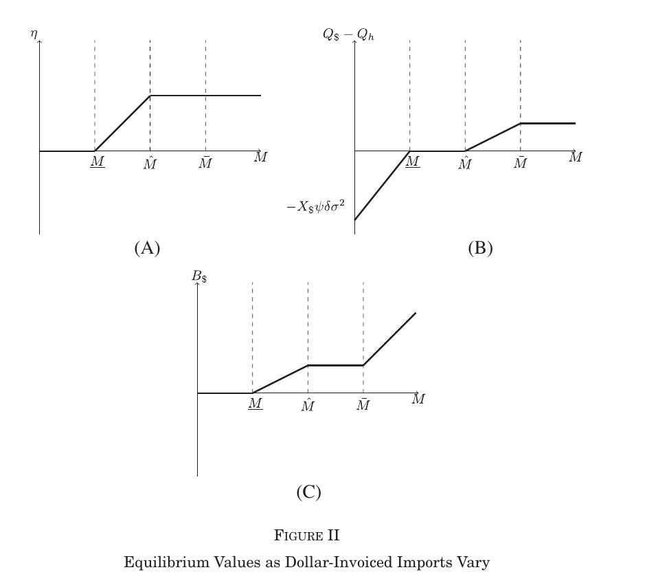
Put the two halves together and Proposition 3 (p. 803) partitions the world by $M$, the volume of dollar-invoiced imports. Below $\underline{M} = X_\text{USD}$, Treasuries cover everything and nobody invoices in dollars. Between $\underline{M}$ and $\hat{M}$, exporters convert just enough to keep the premium at exactly zero — interior invoicing, precisely because the price is pinned. Above $\hat{M}$ the export projects are exhausted, the premium reopens, and it climbs until it hits its ceiling $\theta(\bar{\mathcal{E}}-1)$ at $\bar{M}$, where $\theta = \delta - \beta$ is the safety premium households pay. Only past $\bar{M}$ do banks start drawing on home-currency projects to back dollar deposits, which is the mismatch region. That the ceiling is a ceiling — that the premium never has to rise further — is because the first unit of currency conversion costs a discrete amount proportional to $\bar{\mathcal{E}} - 1$, so once you’re paying that you can convert as much as you like.

Two currencies, and why the world only wants one

Now put a continuum of emerging markets in a ring around a United States and a Europe that are identical in every parameter, and let each country’s dollar-invoiced imports be $M_{\text{USD}i} = a + b\int_{j\neq i}\eta_j\,dj$ — an exogenous anchor $a$ of always-dollar-priced American exports, plus a feedback term in what everyone else chose. The complementarity is now explicit: more dollar invoicing elsewhere raises your dollar import bill, raises your dollar deposit demand, cheapens dollar funding, and makes your own exporters invoice in dollars.

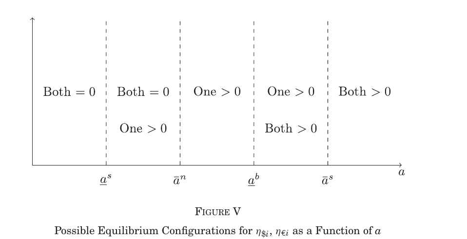
Proposition 5 (pp. 815–816) then says that provided the feedback coefficient $b$ sits inside a stated band, the parameter space in $a$ splits into five regions, and in the middle one the asymmetric single-dominant-currency equilibrium is the unique stable outcome. Which currency dominates, the model refuses to say — they are identical. The economics of the middle region is stated plainly: “while there is enough safe-asset demand to sustain one global currency, there is not enough to sustain two.”

The stability argument underneath that is doing more work than it looks, and it is the paper’s strangest structural result. Because invoicing is bang-bang, a two-currency equilibrium needs $Q_\text{USD} = Q_{\text{EUR}}$ exactly. In the no-mismatch region both prices respond to what other countries do, so an infinitesimal tilt toward the dollar raises $Q_\text{USD}$, breaks the equality, and sends every exporter to a corner — those equilibria are unstable. In the mismatch region $Q_\text{USD}$ is pinned flat at $\theta(\bar{\mathcal{E}}-1)$, independent of what anyone else invoices, so the symmetric equilibrium survives. Stable coexistence of two global currencies therefore requires, in this model, that emerging-market balance sheets carry mismatch in both. A tidy world of two safe reserve currencies and no one bearing currency risk is not somewhere you can stay.

The numerical example, and a small discrepancy in it

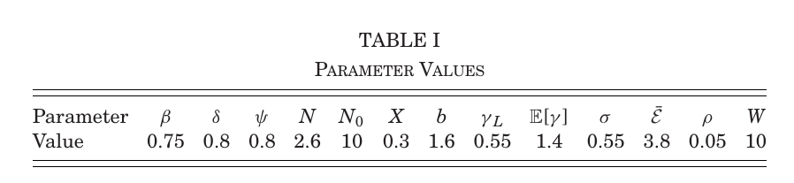
Table I supplies illustrative values, chosen to reproduce the cutoff ordering of Figure V rather than to match data moments. From them, $\theta = \delta - \beta = 0.05$ and $\bar{\mathcal{E}} = 3.8$, so the ceiling on the dollar premium is $\theta(\bar{\mathcal{E}}-1) = 0.14$, which is exactly the plateau you see plotted.

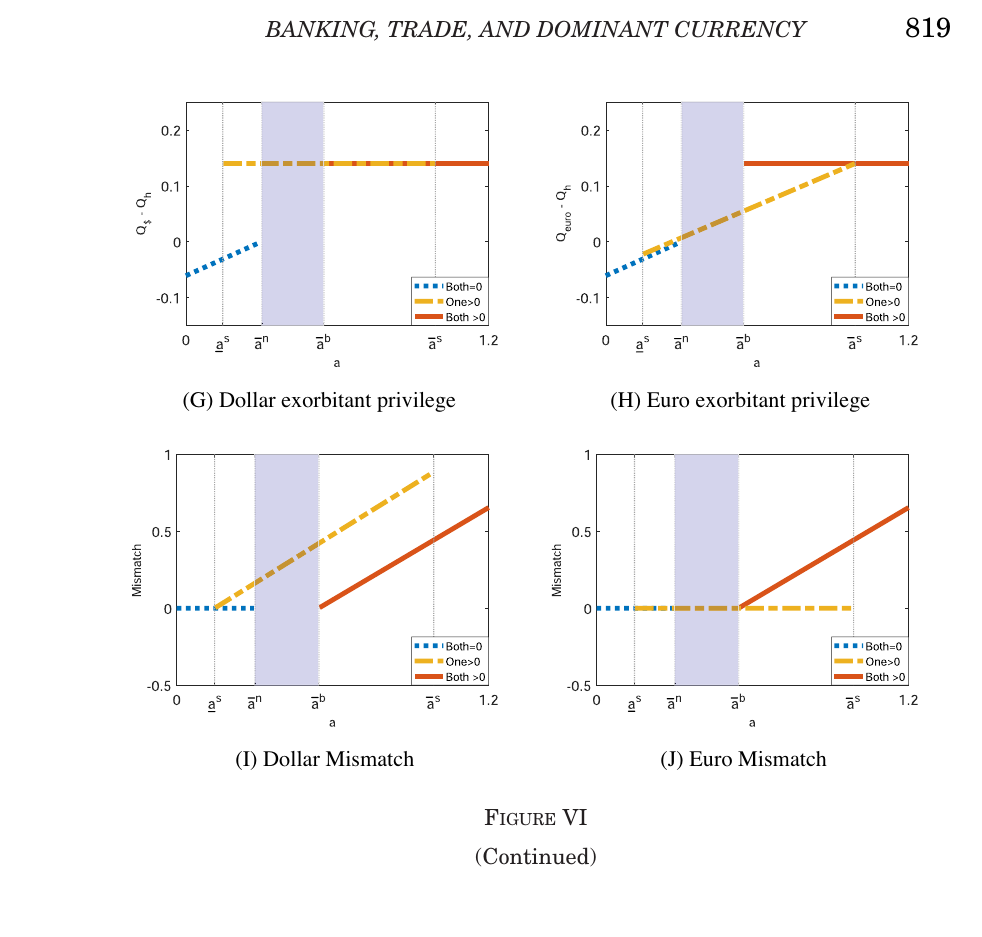
The payoff picture is the asymmetry manufactured out of symmetry. Along the single-dominant-currency branch the dollar premium sits at its ceiling of 0.14 and dollar mismatch grows, while the euro premium is still climbing from below zero and euro mismatch is flat at nothing. Note the nice detail in Panel H: the euro premium turns positive along that branch and still nobody invoices in euros, because what matters is not whether euro funding is cheap but whether it is cheaper than dollar funding, and it isn’t. Two currencies with identical fundamentals, one of them running the world’s collateral factory.

And now the small thing. If you take Table I’s numbers and put them back into Proposition 5’s own printed condition on the feedback coefficient — the one under which the five regions exist at all — they do not satisfy it. The condition requires $b$ above roughly 2.15 at these values; Table I prints $b = 1.6$. (Reading $\sigma = 0.55$ as a variance rather than a standard deviation still leaves a required $b$ of about 1.83, so that isn’t the escape.) Worse, plugging Table I into the printed cutoff formulas reverses the ordering that Figure V asserts and Figure VI draws. Measured off the rendered page, Figure VI’s four region boundaries sit at about 0.15, 0.30, 0.55 and 0.99 — the second of which is $\bar{a}^n = X = 0.3$, exactly as the formula says — but the printed formulas at Table I values put the first boundary above the second, not below it.

There is a reconstruction that fits, and it should be labelled as one, because it is ours and not the paper’s: taking the published two-currency importer problem, carrying the printed correlation $\rho = 0.05$ through it, and setting $\gamma_L N = 0.715$ — precisely half of the 1.43 that Table I’s $\gamma_L = 0.55$ and $N = 2.6$ imply — reproduces all four drawn boundaries to within a pixel, and also reproduces the slope of the plotted single-currency branches, which is 1.05 rather than the 1 the zero-correlation formulas would give. Whether the factor of two lives in a table entry, in the figure code, or in some presentation choice cannot be settled from the article; the replication files are on Dataverse and would presumably settle it, and were not consulted here. What matters is what this does and does not touch. It does not touch a single proposition. The propositions are conditional statements — if $b$ lies in this band, then the cutoffs order this way — and they are unaffected by a numerical illustration that sits outside the band. It is an inconsistency in the picture, not in the theorem, in a paper that has been cited a great deal and re-derived by approximately nobody.

The one that inverts a policy argument

Here is the result that ought to make a European official put down their coffee. The paper reports (p. 822, from an online appendix not in hand here) that as the relative supply of safe assets rises for a country, all else equal, this reduces its ability to become a dominant currency. More euro safe bonds, with no change in the demand for them, means higher euro interest rates, which means emerging-market banks have less reason to manufacture euro safe claims and emerging-market exporters have less reason to invoice in euros. The authors state the inversion themselves and bound it carefully: “It has often been argued that issuing a euro safe bond can help with internationalization of the euro. Interestingly, in the context of our model if such an issuance does not increase the demand for euro safe bonds it does not help with internationalization.” The conditional is load-bearing — if the issuance also raises demand, the argument doesn’t apply. But taken on its own terms it says something counterintuitive about what dominance is made of: the official supply of a safe asset can crowd out precisely the strained, mismatched private intermediation that entrenches a currency. The privilege is downstream of somebody being uncomfortable.

The evidence, which the paper describes as preliminary

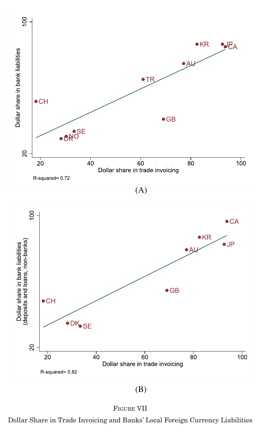
Invoice shares from Gopinath (2015) against the dollar share of banks’ foreign-currency local liabilities from the bis, excluding the eurozone and the us so as not to pick up own-currency use, and excluding Brazil and India for their restrictions on private foreign-currency deposits. That leaves ten countries and an $R^2$ of 0.72; restricting liabilities to deposits and loans from non-banks, to strip out interbank funding, leaves eight countries and 0.82. Switzerland, Denmark, Norway and Sweden sit in the low corner on both axes, which is what you would expect of countries whose trade is with the eurozone. The authors call the contribution “primarily theoretical” and the evidence “preliminary,” and they are right on both counts: this is a cross-section of ten points with no controls, on two variables the theory itself says are jointly determined. It is consistent with the model. It is consistent with several other things too, and the paper says so.

A reconstructed referee report

There is no discussant and no recorded Q&A for this paper; what follows is a reconstruction of where a referee would press, with pointers to where the published text meets the objection.

The first push is on hedging. If the exporter merely wants dollar revenue, why price in dollars instead of pricing at home and buying a forward? Unbundle the goods-pricing decision from the risk-management decision and the invoicing channel evaporates. Remark 3 (pp. 804–805) is the answer, and it is a good one: hedging requires posting collateral, which is expensive exactly for the liquidity-constrained firms in question, and invoicing in dollars sources the hedge from a counterparty who is already fully protected — the Brazilian importer “does not have to turn over any cash until it receives its machines and is not promised anything other than the machines in any state of the world,” unlike a derivatives dealer who pays out in one state hoping to collect a default-prone payment in another. It is narrated rather than modelled, though; the hedging cost never enters an optimisation, so the paper cannot say how large it must be for the result to hold.

The second is that a uip violation in a mean-variance model with a fixed expected exchange rate is close to a definition, and that the size of the privilege depends on nothing but the worst-case exchange rate $\bar{\mathcal{E}}$. The authors concede both halves. Remark 1 (p. 798) says the model is “best thought of as suited to making on-average statements” and disclaims any high-frequency implication, including the forward premium puzzle. Footnote 9 calls the $\bar{\mathcal{E}}$-dependence “somewhat unnatural” and offers a reinterpretation in which the collateral constraint proxies capital regulation and the relevant object is a tail moment — an honest concession that costs them Proposition 1’s clean ratio.

The third is that the whole selection story rides on linearity. Invoicing jumps from zero to one the instant the premium turns positive, and that is exactly what makes no-mismatch dual-currency equilibria unstable. Footnote 15 points to the 2018 working paper, where an ad hoc friction makes the invoicing share continuous with qualitatively similar results — but that is a pointer, not a demonstration in this document, and the instability argument in Section V is precisely where the corner solution is doing the most work.

And the fourth is the calibration described above, which is real, checkable on the printed page, and confined to the illustration.

Where it sits

This is the theory slot in section 3.1 of the geoeconomics list, presented rather than cited, and presented because it is the foundation of the currency-dominance and sanctions-finance sub-block rather than one of its applications. Every paper the group will read about weaponized finance assumes that invoicing, bank funding, corporate borrowing and reserves are one system rather than four literatures; this is the paper that shows why they have to be. It is also what makes the rest of the list cohere. Dollar Dominance and the Transmission of Monetary Policy (McLeay and Tenreyro 2026) and Mukhin’s (2022) price-system model take the invoicing leg. Farhi–Maggiori (2018), Bianchi–Sosa-Padilla (2025) and Global Hegemony and Exorbitant Privilege (Pflueger and Yared 2024) take the reserve-asset leg and ask what the hegemon can charge for standing behind it. Bahaj–Reis (2022) on swap lines and Internationalizing Like China (Clayton et al. 2025) are attempts to start the loop for a second currency, which this model says means crossing a threshold rather than nudging a share. Eichengreen–Mehl–Chiţu’s (2017) alliance effect is the history the indeterminate region leaves room for.

The reason to put it on the board first, even for a group that has met it, is the shape of the discontinuity. Invoicing here jumps from zero to one; it does not drift. And that shape is sharper in the published version than in the 2018 draft, which is what referee reports are for. If you take the model seriously, “de-dollarization” is not a number that declines. It is a region you either enter or don’t, and the paper’s own equilibrium-selection rule — go back to the last date at which the model pinned things down uniquely, and stay there until the parameters make it untenable — says the incumbent gets the benefit of the doubt for a long time. Europe catching up with the United States, the authors suggest, might not be enough; it might take Europe getting substantially bigger. Which is a curious thing to conclude from a model in which the two are, by construction, identical.

References