Notes on:

The Fiscal Implications of Parallel Currencies

Saleem Bahaj & Ricardo Reis
Unpublished working paper, August 2026
1 August 2026
offshore currency · capital controls · seigniorage · exchange rate policy · integrated policy framework · CNH
Paper · PDF
Haiku 4.5 (research), Opus 5 (reading, figures, diagram and writing), GPT 5.6-Sol (reading), Fable 5 (adjudication), GPT 6-Astra (verification)

Saleem Bahaj (ucl) and Ricardo Reis (lse), “The Fiscal Implications of Parallel Currencies,” August 2026. Unpublished working paper — no journal, no doi. Written from the August 2026 draft alone; there is no recorded talk, no discussant and no Q&A, so everything below that reads like an objection is my own reading, not anyone’s reported remark.

You run a small open economy and would like to lean against capital flows. The ipf offers you a Tobin tax, which has the problem Brazil discovered: gross flows somebody has to identify, a rate you cannot move at high frequency, an evasion margin at every accounting seam. Brazil went to 6% in 2010 and collected 0.05% of gdp.

So you do it sideways. Forbid direct cross-border claims in both directions, and permit exactly one instrument that crosses: a bank deposit in an offshore version of your own currency, issued by banks whose reserves you supply. Now you set a quantity of reserves and the market produces the rate. Bahaj and Reis (2024) proved these are the same policy — same equilibrium exchange rate, one instrument fixing the rate, the other the money supply. This paper asks what that leaves hanging: if it is a tax, who collects, and how much?

The chokepoint

![Schematic of the offshore parallel-currency regime. A thick black wall labelled “capital controls” runs down the middle, separating a “domestic economy” on the left from the “rest of the world” on the right. The wall has one wide opening, filled by a box labelled “Offshore bank — competitive, free entry, zero profit”, carrying D = d-h + d-f, R-d = R(1 - psi(x)), x = M/D, and E = 1 via R-m = R(1 + phi-prime(x)). Top left, a “Domestic household” box holds b-h at R and d-h at R-d and receives T; top right, a “Foreign investor” box discounts at 1/R-dollar and holds d-f at R-d. Hairlines from each box run at the wall and are struck through with a cross, marked “no direct claim abroad” and “no direct claim onshore”. Bottom left, a “Government” box issues M at R-m and B-g at R, holds B-dollar at R-dollar and rebates T; two red arrows run from the bank to it, a solid one labelled minus phi-prime(x) M over beta and a dashed one labelled phi(x) D, jointly marked F(M), fiscal revenue. A single narrow slit low in the wall carries a government arrow labelled B-dollar at R-dollar, captioned “the sovereign’s own window”. On the right, a rate ladder shows three rungs — R (onshore bond), R-d (offshore deposit) and, far below, R-m (offshore reserve) — with a red double-headed arrow spanning the top two rungs labelled tau minus 1, and a panel headed “The wedge” giving (R minus R-d) over R-d = tau minus 1 = psi(x) over (1 minus psi(x)).](figures/tikz_offshore-currency-wedge.svg ‘Schematic drawn for this digest — not one of the paper's own exhibits. The architecture of pdf pp. 4–5, which the paper states in prose and never draws: neither households nor foreigners may hold the other side's liabilities directly, so every private cross-border claim is funnelled through offshore bank deposits, and the government owns the tap. Scarce reserves make the deposit rate R-d = R(1 − ψ(x)) sit below the onshore return, and that relative gap (R − R^d)/R^d = τ − 1 is the Tobin-tax rate the regime charges without legislating one. Symbols are hoverable: every one carries its definition, calibrated value and page.’)

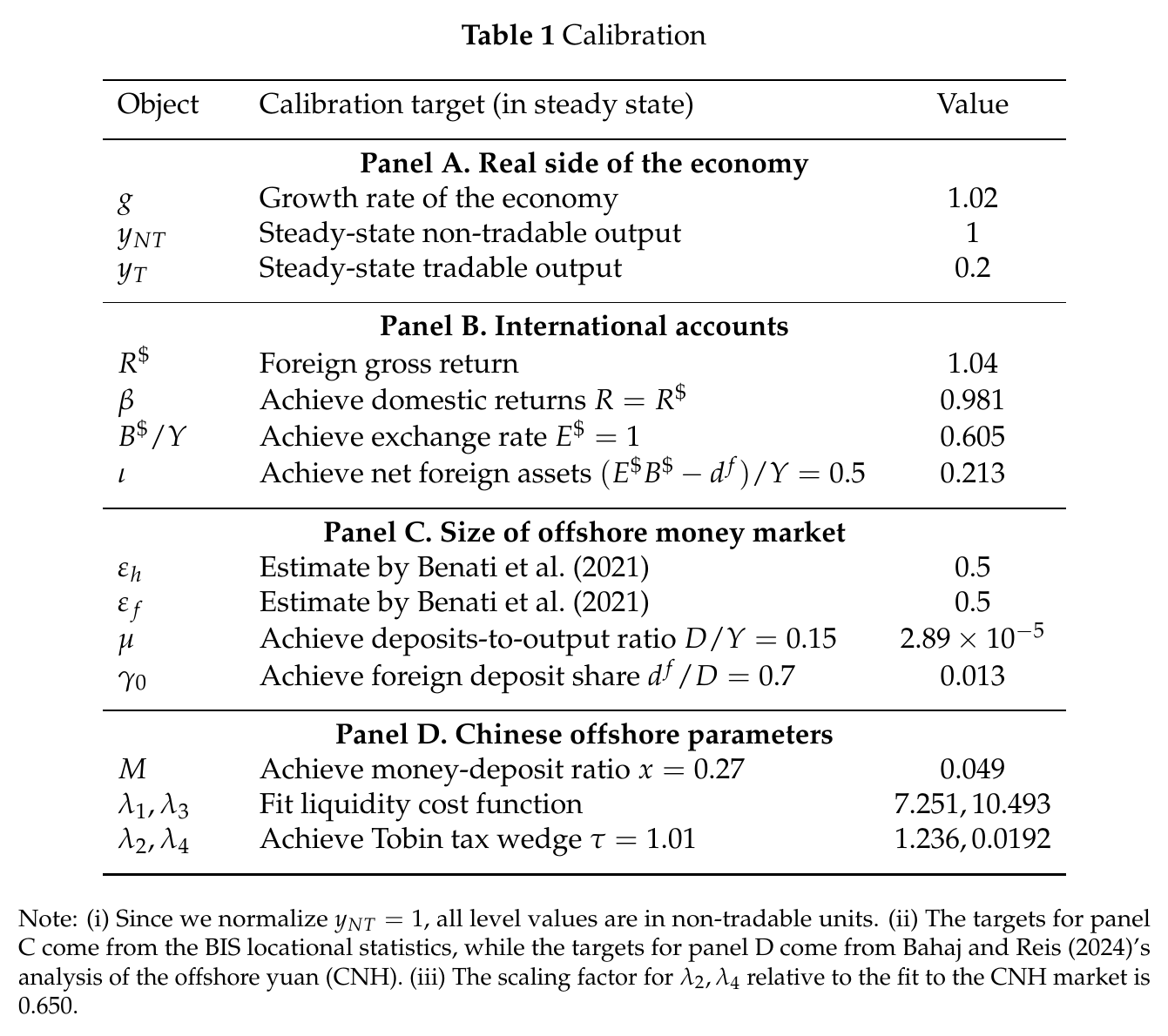
Four agents, one wall, one opening. Households cannot invest abroad, foreigners cannot invest onshore, both may hold offshore deposits; the government supplies offshore narrow money $M$ and is the only agent free to cross. Banks are competitive with free entry, so their liquidity costs land entirely in the deposit rate:

R^d_t = R_t\left(1 - \psi(x_t)\right)

with $x \equiv M/D$ and $\psi(x) = \phi(x) - x\phi'(x)$ the marginal liquidity cost of issuing one more deposit. Scarcer reserves raise $\psi$ and push $R^d$ below the onshore return $R$ . That relative gap is the tax rate, eq. 34 in the paper:

\tau \equiv 1 + \frac{\psi(x)}{1-\psi(x)} \;=\; \frac{1}{1-\psi(x)}

Two sub-wedges ride in there: foreigners can only ever earn $R^d$ , and banks eat $\psi(x)$ when they fund domestic assets. Nobody ever writes down a tax. The Treasury’s revenue is an interest rate it declines to pay.

A rate times a base

Lemma 1 has four budget terms; the paper deletes two (net foreign investment income, debt service) as artefacts of the zero-private-foreign-savings and Ricardian assumptions rather than features of the regime, leaving Definition 1, eq. 33:

F(M) \equiv -\left(\frac{\phi'(M/D)}{\beta}\right)\left(\frac{M}{Y}\right) + \phi(M/D)\left(\frac{D}{Y}\right)

Seigniorage first — reserves pay $R^m = R(1+\phi'(x))$ with $\phi' \le 0$ , so the government keeps the marginal liquidity benefit on base $M$ . Liquidity revenue second — the average per-deposit cost on base $D$ , which in the Bahaj–Reis microfoundation is penalty payments at the lending facility, once interbank legs net out. Different derivative, different base. Then Lemma 2, eq. 35, the whole paper in one line:

F(M) \approx (\tau - 1)\left(\frac{D}{Y}\right)

Four-panel calibration table. Panel A, real side: growth g = 1.02, non-tradable output y_NT = 1, tradable output y_T = 0.2. Panel B, international accounts: foreign gross return R-dollar = 1.04, beta = 0.981 to hit R = R-dollar, B-dollar over Y = 0.605 to hit exchange rate E-dollar = 1, iota = 0.213 to hit net foreign assets of 0.5. Panel C, size of the offshore money market: epsilon_h = epsilon_f = 0.5 from Benati et al. 2021, mu = 2.89 times ten to the minus five to hit deposits over output of 0.15, gamma_0 = 0.013 to hit a foreign deposit share of 0.7. Panel D, Chinese offshore parameters: M = 0.049 to hit a money-deposit ratio x = 0.27, lambda_1 and lambda_3 = 7.251 and 10.493 fitting the liquidity cost function, lambda_2 and lambda_4 = 1.236 and 0.0192 to hit a Tobin tax wedge tau = 1.01. — Table 1, paper PDF p. 21: “Calibration.” Panel C targets come from BIS locational banking statistics; Panel D targets come from Bahaj and Reis (2024) on the offshore yuan, with the two level parameters scaled down by 0.650 so the implied net wedge is 1% rather than the 1.55% the raw CNH fit delivers.

A rate times a base, done on a napkin: 1% times 15% is 0.15% of gdp. Across the bis cross-border deposit ratios (eur 0.167, gbp 0.130, jpy 0.134, chf 0.066) the range is 0.07% to 0.17%; Brazil’s 6% read as a wedge would be 0.9% at best; the cnh itself, the only real instance of the regime, has averaged 0.002%. For scale, this economy’s net foreign investment income — one of the terms the paper discarded — is 1.19% of gdp, almost eight times the revenue it kept.

The press runs backwards

Now vary the instrument. This is Lemma 3, eq. 36, whose Appendix D derivation equates the onshore and foreign gross returns, as the calibration does:

\frac{d\log(F(M))}{d\log(M)} = \left[\eta(x) - \left(\frac{d^h}{D}\right)\varepsilon_h - \left(\frac{d^f}{D}\right)\varepsilon_f\right]\frac{d\log(\tau-1)}{\tau\, d\log M} + \left[\left(\frac{d^f}{D}\right)\varepsilon_f - \frac{E^\$ y_T}{Y}\right]\frac{d\log E^\$}{d\log M}

Two stacked line charts. Panel (a), “The exchange rate and foreign deposits”: the exchange rate E-dollar rises from 0.9983 to 1.0028 as M/Y goes from 0.020 to 0.060, with a top axis showing foreign deposits over GDP rising from 0.096 to 0.123. Panel (b), “Fiscal offshore revenues and the tax wedge”: F over Y in percent falls from about 0.166 to 0.129 over the same range of M/Y, with a top axis showing the net wedge falling from 1.20 to 0.73 percent. Both panels carry a dashed vertical line at the baseline M/Y = 4.1 percent. — Figure 2, paper PDF p. 24: “Varying the supply of offshore money.” Panel (a) is the general-equilibrium channel — more offshore money means more foreign deposits and a depreciated domestic currency; panel (b) is the total Laffer curve, downward-sloping at the calibration because the wedge falls faster than the deposit base grows.

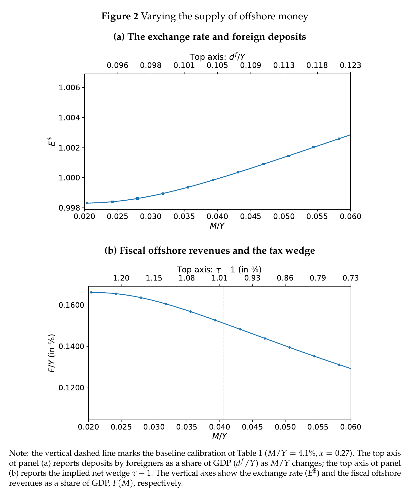
The second bracket is the exchange-rate channel and it behaves: print more, foreigners take more deposits, the currency depreciates, the base grows — weight $0.35$ against the tradables drag $1/6$ . The first bracket is where it goes wrong. At unit elasticity it vanishes, the base shrinking exactly as fast as the wedge rises. At $\varepsilon_h = \varepsilon_f = 0.5$ , lifted from Benati et al. (2021), it is about $+0.5$ and multiplies a negative wedge response. Injecting reserves cuts the scarcity premium by more than it grows the base, and the calibrated economy sits on the downward-sloping side: $M/Y$ from 4% to 6% depreciates the currency 0.29%, drops the wedge 0.28 points, and costs about 0.02 points of gdp; cutting back by the same two points buys only 0.015, because the curve is concave.

That inversion is the thing. In the standard seigniorage problem the government picks the rate and the base responds, and low demand elasticity is what makes a base safe to tax. Here the government picks the base instrument and the market hands back the rate, so the same low elasticity is why the tool works in reverse. Conditional on this calibration and on $\varepsilon = 0.5$ — at $\varepsilon_f = 10$ the curve flips upward, still worth at most an extra 0.05% of gdp from a 50% increase in $M$ — a finance minister who wants more from the offshore printing press has to print less.

Level and slope come from different places

Line chart, share of nominal GDP from 0 to 0.15 percent on the vertical axis against the offshore money supply M over GDP from 0.020 to 0.060 on the horizontal axis, with a second top axis showing the implied net wedge falling from 1.20 to 0.73 percent. A black “Total” line slopes gently downward from about 0.165 to 0.130. A blue dashed “Seigniorage” line rises from 0.118, peaks around 0.142 at M/Y near 0.033, then declines to 0.125. An orange dotted “Liquidity” line falls steeply from 0.047 to under 0.005. A grey dashed vertical line marks the baseline at M/Y = 4.1 percent. — Figure 3, paper PDF p. 26: “Seigniorage and liquidity revenues as the supply of offshore money varies.” The calibrated economy (dashed line, M/Y = 4.1%, x = 0.27) sits on the downward-sloping side of the total Laffer curve; seigniorage is about 93% of the 0.15%-of-GDP total, but liquidity revenue is what drives the slope in the scarce region to the left.

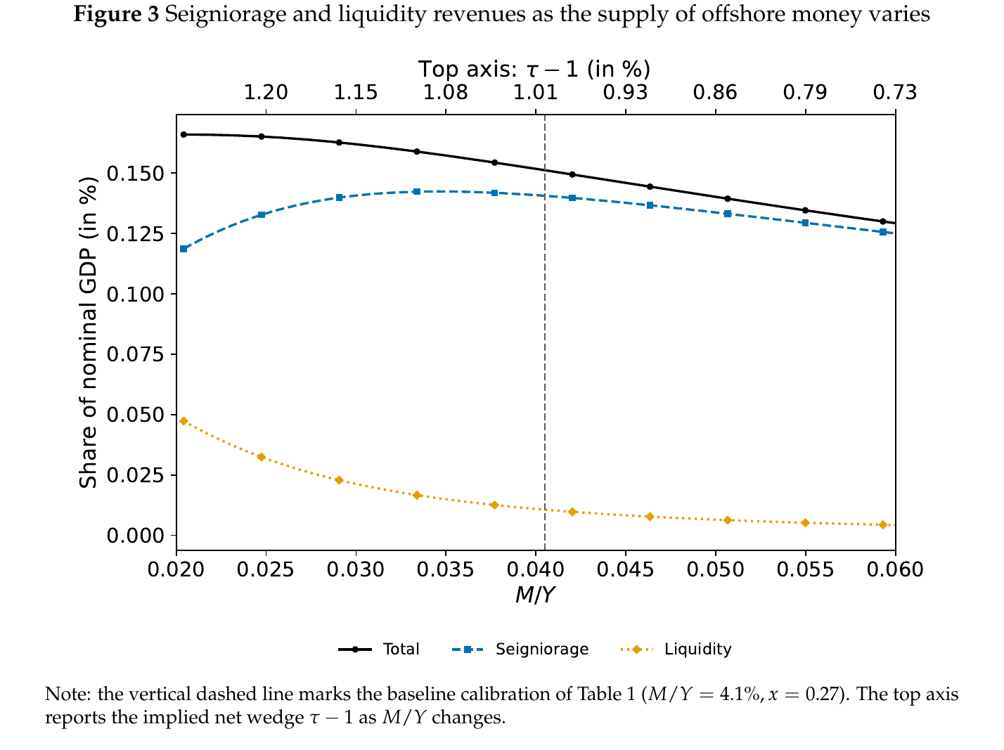
Seigniorage is about 93% of the total, liquidity about 7%, but the two have separate Laffer curves and the seigniorage one has an interior peak: below $M/Y \approx 3.5\%$ , cutting reserves lowers seigniorage while raising liquidity revenue so sharply that the total rises anyway. The level is a seigniorage story, the slope in the scarce region a liquidity story, and over part of the range the total and its dominant component sit on opposite sides of their own peaks. Incidence follows holder shares even though banks make the payment: 70% foreigners, 30% households.

Where this is most exposed

The headline is a calibration target before it is a result. $D/Y = 0.15$ is a round number near the bis ratios, and $\tau - 1 = 1\%$ comes from scaling the cnh-fitted level parameters by 0.650 — down from the raw fit’s 1.55%, but up from the 0.3% wedge Bahaj and Reis (2024) actually estimate for the cnh. Lemma 2 then delivers 0.15% before the model is solved. The defence — transparency and range, and “a representative small open economy,” not China — is a real one. Still: the liquidity technology is fitted visually over $x \in [0.15, 0.4]$ with no standard errors and no out-of-interval validation, the unrescaled 1.55% calibration is never run, and the 75-fold gap between the modelled 0.15% and the only real case’s 0.002% does quiet work in how “small” reads.

Second, every penny of bank liquidity cost is assumed to land in the Treasury. The authors flag it — “this extreme view … biases our fiscal revenues upward, so the small numbers we report are an upper bound” — which defends smallness well and the decomposition badly, since 93/7 is already the most liquidity-favourable split available and liquidity revenue is what drives the total slope in the scarce region. Nothing on the empirical public-capture share, or on operational losses and credit risk at the facilities.

Third, the discarded terms are eight times the kept ones, and one experiment moves them. Fine in the baseline; less fine in Section 5.1, where sterilization is the instrument and government foreign-bond holdings are what changes. Footnote 6 concedes that doubling $M$ under sterilization would raise foreign investment income by 0.1 points of gdp — comparable to the entire offshore revenue — then quarantines it under the assumption that the private sector offsets none of the change in net foreign assets. “Small fiscal footprint” is conditional on an accounting boundary the peg-defence exercise itself pierces.

Then the quiet list, which is the part a peer audience wants. No welfare, anywhere: a wedge borne 70% by foreigners is reported and dropped, when in most open-economy models that is a terms-of-trade transfer and an argument for the regime. “Flat” is a claim about gdp shares, not elasticities — $M/Y$ from 4.1% to 6% is a 46% move in the instrument for about 0.02 of 0.15 points of revenue, roughly 13% (that arithmetic is mine, not the paper’s) — and no revenue elasticity is reported as a number. The controls never leak, in a paper whose opening complaint about Tobin taxes is that they open many paths for evasion, and the Gresham’s-law pressure holding $E = 1$ is asserted, not modelled. No shocks, no transition, no valuation losses on the reserve portfolio — precisely where fx-intervention regimes lose money. And $\varepsilon = 0.5$ is long-run domestic money demand transplanted onto offshore deposits held by deep-pocketed foreigners, with $\varepsilon_f = 10$ the only stress test in the other direction. Market size is the one dimension where the footprint is genuinely not insensitive: doubling deposit demand roughly doubles revenue, so a currency that internationalized far enough could in principle outgrow the smallness result.

One last thing the paper does not say. Look again at Figure 2(a): the revenue-maximizing direction is to contract $M$ , and contracting $M$ is the appreciating direction. The fiscal temptation, small as it is, points toward a tighter offshore market and an overvalued currency — the financial-repression configuration the paper is reassuring us about, reached from the other side. At these magnitudes the reassurance holds. The arrow just points the way it points.

References

Bahaj, Saleem, and Ricardo Reis. 2024. “The Anatomy of a Peg: Lessons from China’s Parallel Currencies.” CEPR Discussion Paper 18749.

Benati, Luca, Robert E. Lucas, Juan Pablo Nicolini, and Warren Weber. 2021. “International evidence on long-run money demand.” Journal of Monetary Economics 117: 43–63. doi:10.1016/j.jmoneco.2020.07.003.