Will The University Endowment Tax Slow Scientific Progress? Evidence from Elite Economics PhD Programs

Joshua Angrist, Marc Diederichs and Glenn Ellison
Presented by Glenn Ellison at the nber Economics of Talent Conference, Cambridge ma, 2 October 2026 (video). No discussant.
Source note: the paper version used is nber Working Paper 35244, May 2026. Several exhibits in the talk are not in that paper: the back-of-the-envelope calibration and the elasticity on the summary slide, the citation regressions, the publication-concentration slides and the cross-field comparison. Each is flagged as talk-only where it appears.

A tax that turns a sorting question into a policy question

The 2025 One Big Beautiful Bill Act raised the private university endowment tax. The top rate is 8%, on schools with more than $2 million of endowment per student, and five schools pay it: Harvard, mit, Princeton, Stanford and Yale (paper p. 1). In the talk Ellison put it more bluntly: “it’s really a tax mostly on five schools who will pay almost 80% of the taxes” (00:46:30), a figure from the talk that the paper does not carry. The schools are responding the obvious way. Harvard has considered halving PhD admissions in many programs, and mit’s institute-wide graduate admissions for Fall 2026 were down 20% (paper p. 1).

Whether that matters for research depends on a question economists normally ask about exam schools and colleges. Is the elite program adding value, or is it a very good sorting machine? If it is sorting, the cut is close to harmless. The student Harvard no longer admits goes somewhere else and takes her talent with her. The paper’s own line: “The University of Michigan Economics Department, for instance, would likely welcome applicants displaced from Harvard to Ann Arbor” (paper p. 8). If it is value added, the cut destroys output, and even then the mechanism matters. If the value is classmates (Ellison: “having talented classmates helps you be productive”, 00:49:40), the displaced stars take it with them when they all land in Ann Arbor together. If it is home journals favouring their own (the qje at Harvard, the jpe at Chicago, aea Papers and Proceedings run by elite officers), the private loss to the students is real and the social loss is small.

So the paper has three jobs. Separate value added from selection, then check that the value added is not peers, and then check that it is not editors.

MIT’s finalist files

Ellison, who is also one of the conference’s organisers, presented with both coauthors in the room. The data are the paper’s real asset. At mit each economics PhD file is read first by one or two faculty members, and the promising ones go to a wider committee whose readers all rate them. The sample is those finalists, 150 to 200 a year, for the 1996–97, 2005–10 and 2012–19 cohorts: 2,582 applicants in all (paper p. 4). Ratings are averaged across readers and turned into a within-cohort rank. That rank is a preliminary judgement, not the admission decision, which also weighed funding and field balance. Ellison: “mit at the time only had funding for about half the students. So, they were often going down to rank 100, 150, 200 to get students who brought their own funding with them” (00:54:16). This gap between rank and admission is part of what the design uses: students of the same rank end up at quite different schools.

Careers are tracked from EconLit dissertation records, department records and cvs, and publications run through 2024. The main outcome is “weighted di” (wdi). It counts publications in 137 “deep impact” journals, each weighted by how often the top five cite it and normalised so the average top-five article counts one, with 1/n credit for an n-author paper. aej: Applied gets 0.44, jep 0.30, aej: Policy 0.24 (paper p. 5). A four-author qje paper, Ellison pointed out, is worth 0.25, so a wdi of two means “you’ve done a lot of publishing” (01:00:06).

The committee could see it coming

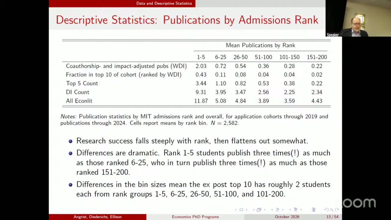
This is the result I would take home. These 2,582 people are already the top of a very strong pool; mit, Ellison noted, gets more than 200 applicants a year with a perfect quantitative gre. Even so, a few faculty reading folders sorted them with remarkable power. Applicants ranked 1–5 average 2.03 wdi publications and those ranked 151–200 average 0.22. Rank 1–5 applicants have a 43% chance of ending up in their cohort’s ex-post top 10, and rank 151–200 applicants have 2%. The typical rank 1–5 applicant ends up with 3.44 top-five papers, counted without any coauthor discount (Table 1). Asked what made the top five so special (01:02:24), Ellison gave the unglamorous answer. Some had an undergraduate thesis about to come out in Econometrica. Others had taken Harvard PhD courses and got A+ grades, or had written papers that were “observably very good” (01:02:43).

The predictability has a limit, and the paper is careful about it. The low-rank bins are much bigger, so the ex-post top 10 holds about two applicants each from ranks 1–5, 6–25, 26–50, 51–100 and 101–200 (paper p. 7). Most of the stars come from rank 26 or worse. Conditional on school, cohort and rank, the pseudo-$R^2$ is at most 0.35 (paper p. 17; Table 5). Ellison’s summary: there can be “large predictable components of success… large differences in value added across schools… a large unpredictable component. All three of these things can be true simultaneously” (01:05:18).

The predictable component is the problem and also the cure. It is the problem because rank 1–5 applicants go mostly to mit, Harvard and Stanford, so raw school gaps are full of selection. It is the cure because the thing that predicts success is in the data.

A value-added model with one control that matters

The framework is Angrist’s value-added setup from the school literature, made exponential because publication counts are non-negative. The identifying assumption is selection on observables in the style of Dale and Krueger:

Here $\nu_i^k$ is applicant $i$’s unobserved productivity shifter for outcome $k$, $D_i$ is the vector of school-attended dummies, and $X_i$ holds the controls (functions of mit rank, the mit-admit and nsf-fellowship dummies, and for 2013–19 the list of schools applied to). That delivers a causal conditional expectation function:

Here $Y_i^k$ is publication outcome $k$, and $e^{\beta_j^k}-1$ is school $j$’s proportional value added relative to the omitted group. In the grouped version $\sum_j D_{ij}\beta_j^k$ becomes $\alpha + \beta_1 T_{1i} + \beta_2 T_{2i} + \beta_f F_i$, where $T_1$ is the high-tax five, $T_2$ is Berkeley, Chicago and Northwestern, and $F$ is foreign schools. The omitted group is the other us schools: Columbia, Penn, nyu, Michigan and so on. Estimation is Poisson pseudo-maximum likelihood with robust standard errors (01:08:33).

Ellison introduced the controls with a taxonomy he credited to Angrist: “They’re bad controls. They’re good controls. They’re awesome controls… when you have awesome controls, they make all the other controls irrelevant” (00:50:31). It is a joke, and it also describes the result. Of everything in $X_i$, only the reciprocal of rank does any work. In the wdi regression with controls, 1/Rank has a coefficient of 1.70 (se 0.24). The linear and quadratic rank terms, the mit admit dummy and the nsf dummy are small and insignificant in every specification (paper p. 11; Appendix Table A1). The reciprocal is steep at the top and flat below, which is exactly the shape of Table 1.

The answer: about 75%

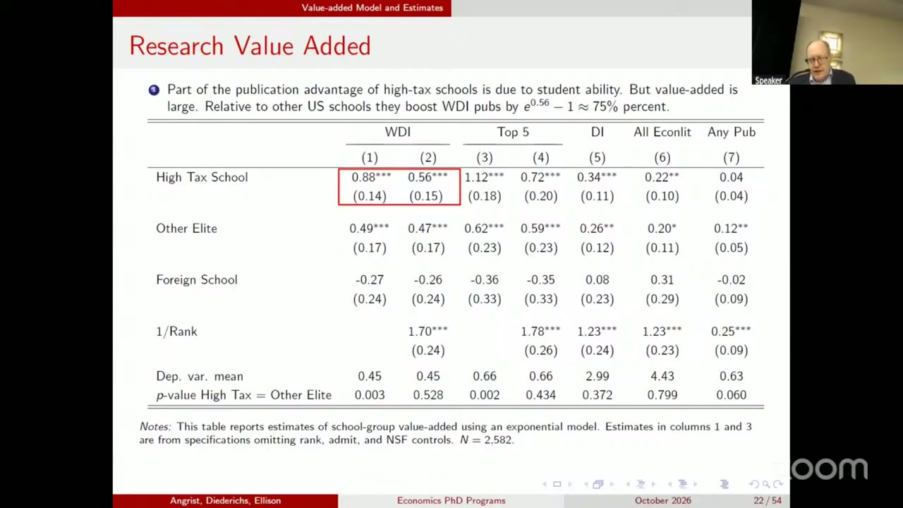
Without rank controls the high-tax coefficient on wdi is 0.88, a 141% gap over other us schools. With them it is 0.56, or 75% (Table 2, paper p. 10). On top-five counts the drop is from 1.12 to 0.72, which still means about twice as many top-five papers. So, in Ellison’s accounting, about half of the raw 141% is selection, and the half that survives is large.

The other elite three do something stranger. Their coefficient barely moves, from 0.49 to 0.47, about 60%. The reason is that Berkeley, Chicago and Northwestern enrollees were ranked much like the students who went to Columbia, Penn, nyu and Michigan (paper p. 11). Those three schools get comparable students and turn out about 60% more weighted output. Without controls the high-tax and other-elite coefficients differ clearly (p = 0.003); with controls they do not (p = 0.528). A few minutes later Angrist made a remark the captions lost, and the reply, apparently Ellison’s, pointed back at this slide: with controls, 0.56 and 0.47 are numbers “we’re not able to statistically say those are different from each other” (01:15:47).

The premium comes mostly from where students publish, not from whether they publish. The all-EconLit coefficient is 0.22, about 40% of the wdi coefficient, so roughly 40% of the premium is more papers and 60% is better journals (paper p. 10). Ellison: “the 56 points is coming say 22 from boosting the number of publications and then 34 from shifting” (01:12:09). On the dummy for publishing anything at all, the high-tax effect is 0.04 with a standard error of 0.04, indistinguishable from zero.

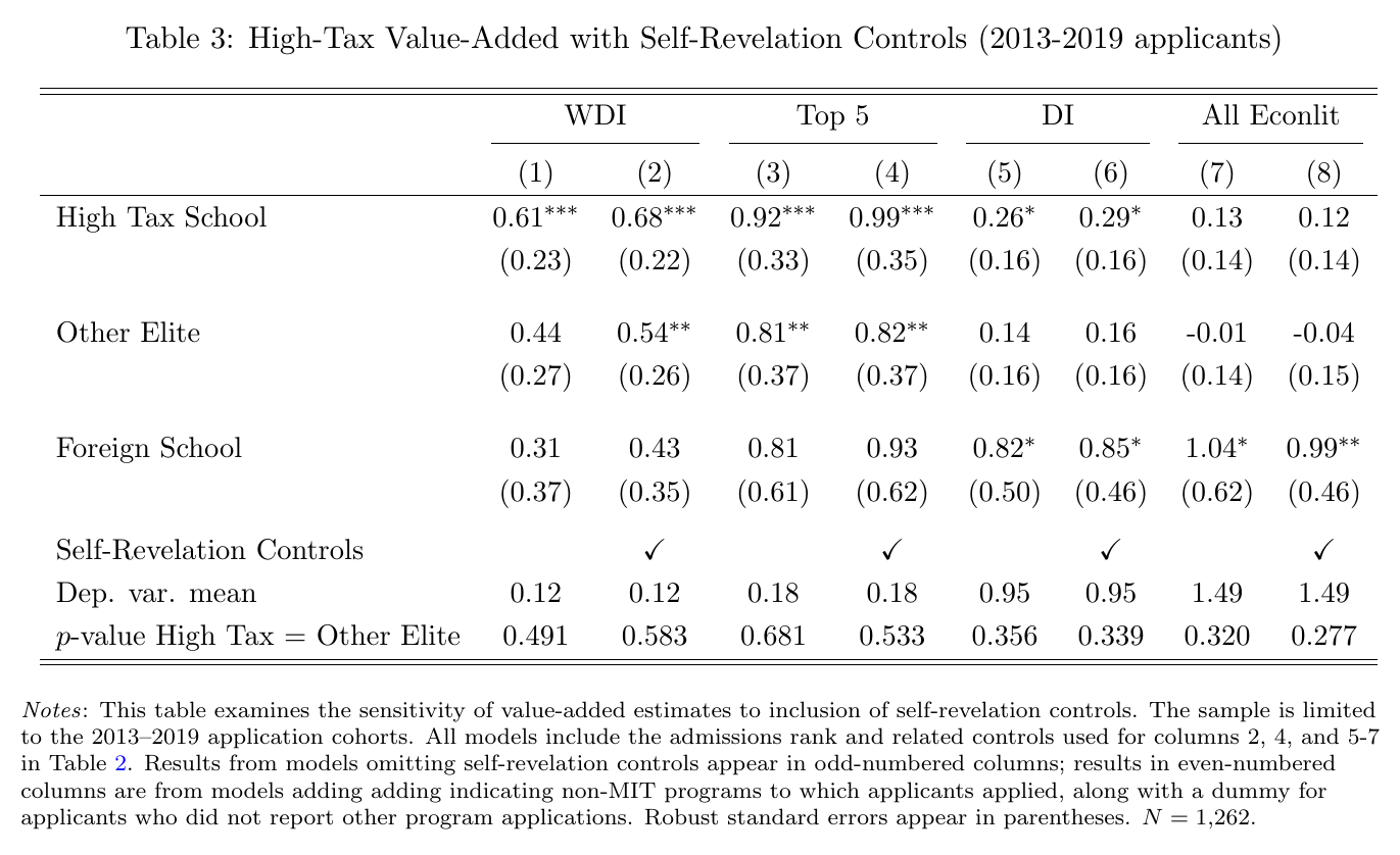
The obvious worry is that rank misses ambition. For the 2013–19 cohorts the authors can add Dale–Krueger “self-revelation” dummies for every other program the applicant applied to, 69 schools in all; 85% also applied to Harvard and 41% to Northwestern (paper p. 11). The high-tax wdi estimate goes from 0.61 to 0.68 and the other-elite estimate from 0.44 to 0.54 (Table 3). Adding the controls, as Ellison put it, “if anything, it actually makes the value added estimates larger” (01:16:38). One caveat: these are recent cohorts with short publication windows and a wdi mean of 0.12, so the check rests on early-career output. (The slide also cites an Oster-style stability analysis that the paper’s main text does not report.)

Not peers, and mostly not the QJE

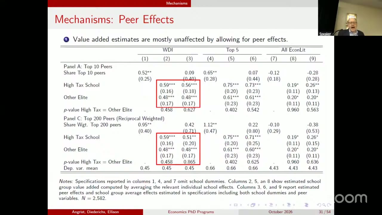
Peer effects are identified from year-to-year swings in who enrolls where. mit got two of its rank 1–10 applicants in 2010 and all of them in 2016; Yale went from three rank 1–150 enrollees in 2016 to 16 in 2017 (paper p. 12). Without school dummies, the share of top-10 classmates looks like it matters: 0.52 for wdi. With school dummies it falls to 0.09 with a standard error of 0.40. The high-tax value added goes from 0.59 to 0.56, or to 0.51 with the reciprocal-weighted peer measure (Table 4). (These group effects are averages of school dummies, which is why they differ slightly from Table 2’s 0.56.) Someone suggested trying top-five peers (01:19:08). Ellison said the reciprocal weighting already “is tipping it a lot towards a top five or 10 peers”, and that peer effects only look large when the school effects are left out. So the cheap fix, sending the displaced stars to Michigan as a group, does not look like it would carry the premium with them.

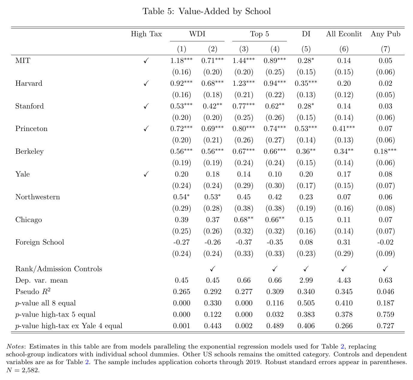
School by school, the rank controls mostly cut down mit and Harvard, whose top-five coefficients fall from 1.44 to 0.89 and from 1.23 to 0.94. Stanford falls less, and the other five barely move (Table 5). Endowment and value added do not line up neatly. Yale is in the top tax bracket and has the smallest wdi estimate, 0.18 with a standard error of 0.24. On wdi, Berkeley (0.56) and Northwestern (0.53) sit a little above Stanford (0.42). On top-five counts Northwestern is below Stanford and Berkeley only just above. Equality of all eight controlled wdi estimates is not rejected (p = 0.330), but with school-level standard errors around 0.2–0.3 that is a failure to reject, not a finding of equality. The paper still allows itself a policy line: high-tax schools “might benefit by emulating features of successful graduate programs at relatively low-endowment elite competitors like Berkeley and Northwestern” (paper p. 17).

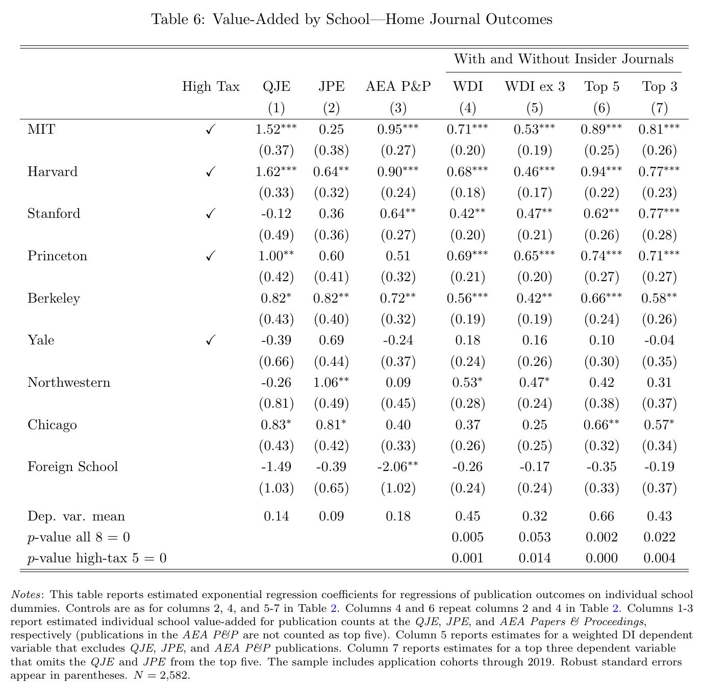
Then the editors. The qje coefficients are large exactly where you would expect: Harvard 1.62, mit 1.52 (Table 6). Ellison’s reading was that if you “send one to Harvard, one to Stanford, the Harvard student publishes five times as many qj papers” (01:20:58). The five is right but the comparison school is mislabelled. $e^{1.62} \approx 5.1$ is Harvard relative to the omitted other-us group. Against Stanford, whose qje coefficient is −0.12, the point estimate is $e^{1.74} \approx 5.7$, and with standard errors of 0.33 and 0.49 that gap is loosely pinned down. On the jpe, Ellison spoke of an “enormous effect of going to Chicago” (01:21:12). The table is more muted, with Northwestern at 1.06 ahead of Berkeley at 0.82 and Chicago at 0.81, and the paper calls the jpe “less of a local success story than the qje” (paper p. 16).

What matters is what happens when you remove those journals. Set the qje, jpe and P&P weights to zero and mit’s wdi estimate goes from 0.71 to 0.53, Harvard’s from 0.68 to 0.46, and the high-tax five are still jointly significant (p = 0.014). Drop the qje and jpe from the top five and Stanford’s estimate actually rises, from 0.62 to 0.77. Part of the Harvard–mit advantage is the home journal, and most of the elite premium survives without it. A talk-only slide adds that elite graduates’ papers are cited more than other papers in the same journal-volume-year, which argues against editors waving through weak papers. Ellison said this of “the high tax and other elite schools” (01:22:51); his slide supports it for the high-tax five and shows roughly nothing for the other three.

Five percent (talk only)

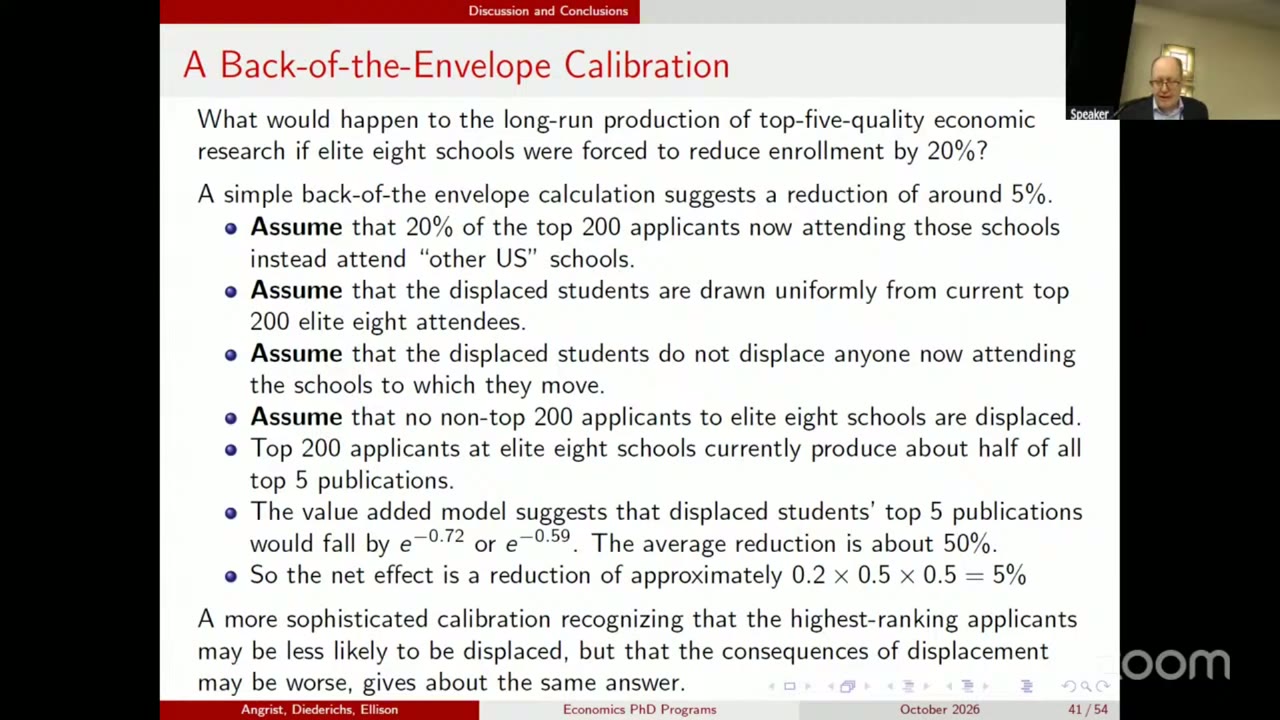
The policy number is not in the paper; it appears only on this slide. Suppose the elite eight cut enrollment by 20%, and 20% of their top-200 students, drawn at random, go to other us schools instead, displacing nobody. The top 200 at elite schools produce about half of all top-five papers. A displaced student’s top-five output is multiplied by $e^{-0.72}$ or $e^{-0.59}$, roughly halved. So 0.2 × 0.5 × 0.5 is about 5% fewer top-five-quality papers across the profession. The summary slide restates this as an elasticity of about −0.25 with respect to high-tax enrollment. The “about half of all top five publications” step carries the most weight and is the least documented. During this slide someone apparently asked about the denominator, and the answer, almost certainly Ellison’s, was that “our top 200 people we know where they all went to school… We don’t know where everyone went to school” (01:23:15). Ellison framed the result as the planner’s trade-off: cut 20% of enrollment, lose 5% of long-run top-five research, “What do we think of that as the tradeoff?” (01:23:57). He then claimed, also only in the talk, that other fields are concentrated enough for the same logic: “it’s not 75% but it is 50 or 60 or something percent” (01:24:10).

What the room pushed on

Questions came throughout. The first was whether publications are a clean measure of output or carry the signalling value of the PhD school (00:52:39). Ellison said they treat publications mainly as output and come back to favouritism later, which they did in Table 6. A sharper version came at 01:03:08: isn’t top-journal success circular, and could an llm judge important research without leaning on the top five? Ellison liked the idea. He pointed to the citation result, and conceded “we think there definitely is sort of some sort of insider bias here” (01:04:19). Asked to put the coefficient in dollars (01:13:10), he said they had not yet done either the private-salary calculation or a welfare-versus-tax-revenue one: it “probably would be something good for us to add to conclusion.” On heterogeneity, splits by citizenship and gender are mostly insignificant, and of a rank-by-school interaction model Ellison said “we’re not finding anything more significant than that” (01:14:43). A garbled question seemed to ask what lies behind the ranks. The answer was that the data hold only the ranks. The authors no longer have the admissions files, so they cannot have a model read them and explain why a student was ranked highly (01:15:06).

That last answer is a fitting place to stop. The variable that rescues the identification is a few faculty members’ judgement of a folder, recorded as a number, and the folders themselves are no longer available. The same judgement decides what a 20% enrollment cut costs, because committees choose who is left out. In a model with proportional school effects, leaving out a low-ranked applicant loses the fewest papers, since a halving of a small expected output is still small. The calibration slide nods to this: a more careful version, in which the highest-ranked applicants are less likely to be displaced but displacement costs more when it happens, “gives about the same answer.” That the two forces roughly cancel is asserted in one sentence on one talk-only slide. It is the number a planner weighing 20% against 5% would most want to see written down.