Are State- and Time-Dependent Models Really Different?

Fernando Alvarez, Francesco Lippi and Juan Passadore · nber Macroeconomics Annual 2016, vol. 31 (University of Chicago Press, 2017), pp. 379–457 · presented by Lippi at the 31st nber Annual Conference on Macroeconomics, April 2016 (video, about 20 minutes, no discussant or Q&A on the recording) · source: published chapter with appendices

Sticky-price macro tells two stories about why a firm keeps its price fixed today. In one, the firm watches its markup every instant and does nothing because doing something costs a menu cost. It moves the moment the markup gets bad enough. In the other, the firm is not watching. It will look at its costs on some date it chose in advance, and until then it has no idea anything is wrong. The first is state-dependent (sd), the Golosov–Lucas (2007) world. The second is time-dependent (td): Taylor (1980), Calvo (1983), Reis’s (2006) inattentive producer. The two camps have tended to assume they disagree about monetary non-neutrality as well as about microfoundations, and the paper notes that some authors (Mankiw–Reis 2002, Klenow–Kryvtsov 2008) expected information frictions to deliver bigger real effects.

Alvarez, Lippi and Passadore’s answer is that, for small shocks, the question is mostly badly posed. Fit the two models to the same frequency of price changes and the same kurtosis of their sizes, and they deliver the same cumulative output response to a small monetary shock. The friction drops out. The models come apart only on large shocks: the menu-cost economy snaps to flexibility, and the inattentive one doesn’t notice until its next review. The authors then go looking for large shocks in exchange-rate data. They find some evidence, and its statistical significance depends rather a lot on one month in South Korea.

The model: one gap, two gates

Everything runs through one state variable. A firm takes a second-order approximation of its profits, and its only state becomes the price gap $g$: log price minus log static-optimal price. Between adjustments the gap is a Brownian motion with drift, $dg = -\pi\,dt + \sigma\,dW$. Inflation erodes it and idiosyncratic cost shocks jostle it (eq. 6 in the paper). The general equilibrium is Golosov–Lucas’s, and it is chosen for one convenience: log utility in real balances makes the nominal wage proportional to money. A once-and-for-all money shock $\delta$ therefore raises every firm’s marginal cost by $\delta$ and knocks every gap down by $\delta$ at the same instant, with the real rate unchanged. Output is then the real wage scaled by $1/\varepsilon$, so the output response is $(\delta - \mathcal{P})/\varepsilon$, where $\mathcal{P}$ is the price-level response. The whole macro question becomes: after every gap drops by $\delta$, how quickly do firms close them?

That is where the two gates come in. In the sd gate, the firm sees $g$ continuously and adjusts when $g$ leaves an inaction set, paying a fixed menu cost that resets all $n$ of its products at once. With $n = 1$ this is Golosov–Lucas. With $n = 2$ or $3$ it is Midrigan (2011) or Bhattarai–Schoenle (2014). As $n \to \infty$ it becomes Taylor-like staggering with normally distributed price changes. In the td gate, review dates come from a duration distribution that is independent of the gap. At each review the firm pays an observation cost, learns its costs and resets; between reviews it does not even know the money shock happened. Constant spells give Taylor, exponential spells give Calvo or Mankiw–Reis, and a Markov chain in observation costs gives something in between. The defining restriction is not a fixed calendar but the independence of timing from the pricing state. Mixed models, namely Nakamura–Steinsson’s (2010) Calvo+ and a model with both menu and observation costs, sit in the middle. The price-level response is split into an impact jump $\Theta(\delta)$ plus a gradual flow, and the summary statistic is cumulative output $\mathcal{M} = \int_0^\infty \mathcal{Y}\,dt$, the area under the output response.

Result one: on impact, almost nobody moves

Here $\Theta(\delta;\pi)$ is the jump in the price level at the instant of a nominal shock $\delta$, starting from steady-state inflation $\pi$, and $\sigma$ is the volatility of idiosyncratic cost shocks (eqs. 23–24 in the paper, Proposition 1).

The td half is close to a tautology, and the talk makes it vivid with Calvo. If a fraction $\lambda$ of firms reprice each month, then $\lambda/4$ reprice each week, fewer each day, and nobody at the instant the shock lands (00:07:28). The sd half is the clever part, and it overturns an old intuition.

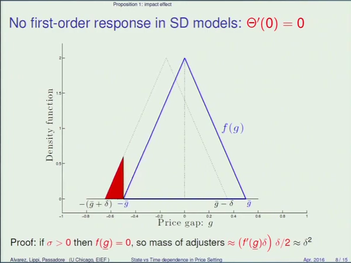
You might think a menu-cost economy has a mass of firms sitting just inside the band, waiting for a nudge, so that a small shock tips a proportional number of them over. It doesn’t, because the band edges are exit points. Any firm whose gap touches the boundary adjusts and leaves, so in steady state no mass can pile up there, and the density at the boundary is exactly zero (Lemma 1; the paper’s discrete random-walk argument shows the boundary density must equal half of itself). Shift the density left by $\delta$ and what falls out is a sliver whose base is $\delta$ and whose height is about $f'(\underline g)\,\delta$. That is a triangle of mass proportional to $\delta^2$. Lippi is careful to say this is a claim about the derivative, not about continuity (00:09:36). So the Caballero–Engel (2007) “flexibility index” is zero in the menu-cost model too, once there are idiosyncratic shocks. The Sheshinski–Weiss (1983) and Caplin–Spulber (1987) results, with their first-order impact, are the $\sigma = 0$ corner, where the density is uniform and mass does sit at the edge.

Inflation matters, but less than you might expect. Higher $\pi/\sigma$ piles density toward the lower edge and makes the sd impact effect larger. At any finite $\pi/\sigma$, though, it is still second order in $\delta$. It becomes first order only in the limit as $\pi/\sigma \to \infty$, which is the Caplin–Spulber world (p. 408). That is the paper’s reason for running its test on low-inflation countries.

Result two: kurtosis over frequency

Here $\mathcal{M}$ is cumulative output, $N$ is the steady-state number of price changes per unit of time, $\mathrm{Kurt}$ is the ordinary (not excess) kurtosis of the size of nonzero price changes, both evaluated at zero inflation, and $1/\varepsilon$ maps real wages into output (eq. 28 in the paper, Proposition 2).

One result could be a curiosity about the first instant. This one covers the whole impulse response. Take any sd, td or mixed model in the class, fit it to the same $N$ and the same kurtosis, and the area under its output response to a small shock is the same, to second order in $(\delta, \pi)$. The friction, whether menu cost, observation cost or a free Calvo opportunity, is absorbed into those two moments. Frequency doing work is unsurprising: an economy that reprices twice as often clears the shock twice as fast. Kurtosis is what Lippi called a summary statistic of how much selection the firms have (00:10:57). Golosov–Lucas, with every price change exactly $\pm\bar g$, has kurtosis 1 and maximal selection: the firms that move are the ones that most need to, so the cpi catches up quickly. Calvo has kurtosis 6 and no size selection at all.

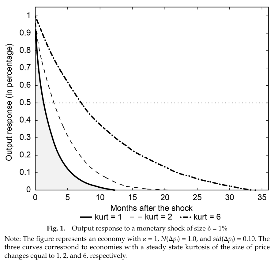
The paper’s Figure 1 shows the economics. It fixes one price change a year and $\varepsilon = 1$, then varies only kurtosis. All three economies start at about 1% extra output, because the cpi does not jump. Read off the plot, their half-lives are roughly 1.5, 3 and 7 months. Plugged into the formula, the areas are about 0.17, 0.33 and 1.0 percent-years. (Strictly, the figure varies kurtosis at fixed frequency; it is not itself a “two different frictions, same moments” exhibit.) The three-model illustration does that job instead (pp. 413–414): a menu-cost model with $n \to \infty$, a pure observation-cost model with constant costs, and a Calvo+ model with 90% free adjustments. All three have kurtosis 3, and so all have the same $\mathcal{M}$. Lippi admitted that at face value they look very different (00:18:23). For the empirical anchor, the authors cite earlier work that puts cleaned micro-data kurtosis near 4, somewhere between Golosov–Lucas and Calvo.

Two pieces of fine print matter. First, equal area is not equal paths: two models with the same $\mathrm{Kurt}/N$ can have differently shaped responses with the same integral. Second, the proof is assembled from pieces. The sd case comes from Alvarez–Le Bihan–Lippi (2016a) and needs $\eta = \rho$ and uncorrelated product shocks. The td case comes from Alvarez–Lippi–Paciello (2016b) and is extended here to $n > 1$ with correlation allowed. The case with both menu and observation costs is checked only numerically, in the appendix.

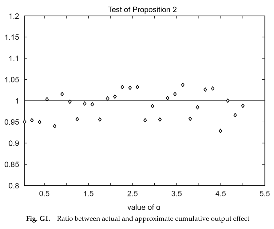
The text says the formula is accurate within ±5% there. The plot itself has several points below 0.95, the lowest near 0.93. That is still a good approximation, just slightly less tidy than advertised.

The one surprising thing

The surprise is that kurtosis also governs the time-dependent model, where by construction nobody selects on their state. Consider Taylor and Calvo calibrated to the same frequency. In both, the firms that reprice after the shock are a random draw, so there is no selection on size. Yet Calvo’s cumulative output effect is twice Taylor’s (p. 411). The reason is selection in timing. Taylor’s spells all last exactly $1/N$. Calvo’s are exponential, with a thick tail of firms that wait a very long time before learning about the shock. And timing dispersion shows up in the size distribution: a long spell accumulates a large gap and a short spell a tiny one. Taylor’s price changes are therefore normal, with kurtosis 3. Calvo’s are a scale mixture of normals, with kurtosis 6. So one number, measured from the cross-section of price changes, captures menu-cost selection on size and inattention-driven selection on timing alike. The authors call this “more surprising” (p. 388). Lippi, by the captions, called it “captured somewhat magically by kurtosis” (00:18:09). A practical corollary: comparing textbook models matched only on frequency gives a misleading contrast, because you have silently fixed their kurtosis at different values.

Result three: big shocks separate them

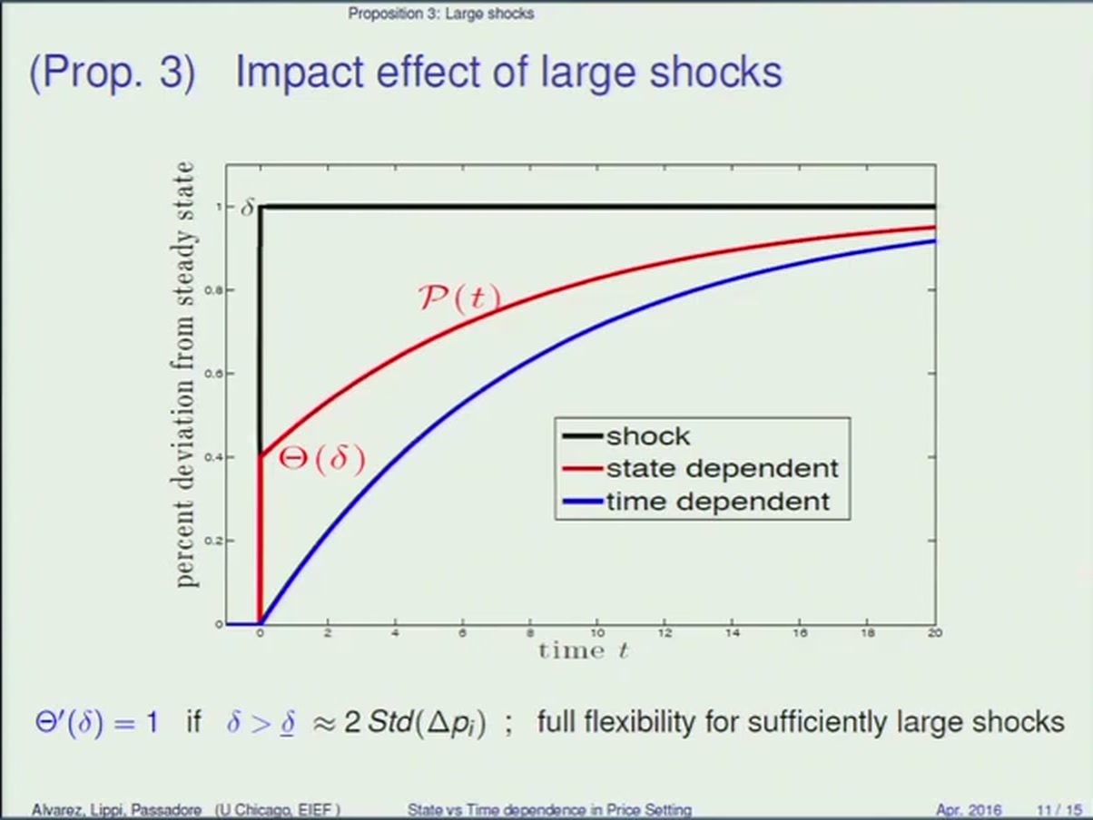
In a td model, $\Theta(\delta) = 0$ for every $\delta$ and the flow is proportional to $\delta$, so $\mathcal{P}(\delta,t) = \delta\,\mathcal{P}(1,t)$. A shock twice as large produces the same response scaled up, with no change in shape. In an sd model the triangle grows faster than $\delta$. Eventually the shifted density lies entirely outside the band, everyone adjusts at once, and money is neutral on impact: $\Theta(\delta) = \delta$ beyond some threshold $\bar\delta(\pi)$ (eq. 33). The “two standard deviations of price changes” rule of thumb on the slide needs its conditions stated. Eq. 32 gives that threshold at zero inflation with $\eta = \rho$ and uncorrelated product shocks. In the single-product, zero-inflation case it is transparent: price changes are $\pm\bar g$, so Std$(\Delta p) = \bar g$, gaps live in $[-\bar g, \bar g]$, and a shock larger than $2\bar g$ pushes every firm out. In Calvo+ the threshold rises with the share of free adjustments and goes to infinity as that share approaches 1, which is what you would expect.

So the paper’s testable prediction concerns curvature: td says the price response is linear in the size of the shock, sd says it is convex.

The evidence: devaluations as money shocks

The authors need many nominal cost shocks of varied size, observed at high frequency, in low-inflation economies. They use monthly imf data on cpi and the end-of-month exchange rate against the dollar (effective rate for the us), 1974–2014. A country-month enters if moving-average inflation is below 8%, gdp per capita is at least $5,000 ppp and population exceeds 2 million. The preferred sample drops pegs, crawling pegs and narrow bands under the Ilzetzki–Reinhart–Rogoff (2019) classification, on the reasonable view that devaluations under a peg are the least exogenous. Then come local projections:

Here $\pi_{i,(t,t+h)}$ is country $i$’s percent cpi inflation from month $t$ to $t+h$, $\Delta e_{i,t}$ is the percent monthly depreciation against the dollar, and $\alpha_i$ and $\delta_t$ are country and month fixed effects (this $\delta_t$ is not the money shock), with $\gamma_h > 0$ as the sd signature (eq. 34 in the paper).

td predicts $\gamma_h = 0$ at every horizon, and sd predicts $\gamma_h > 0$ at short horizons that fades later. The sign term imposes symmetry between devaluations and revaluations; the paper assumes it rather than testing it.

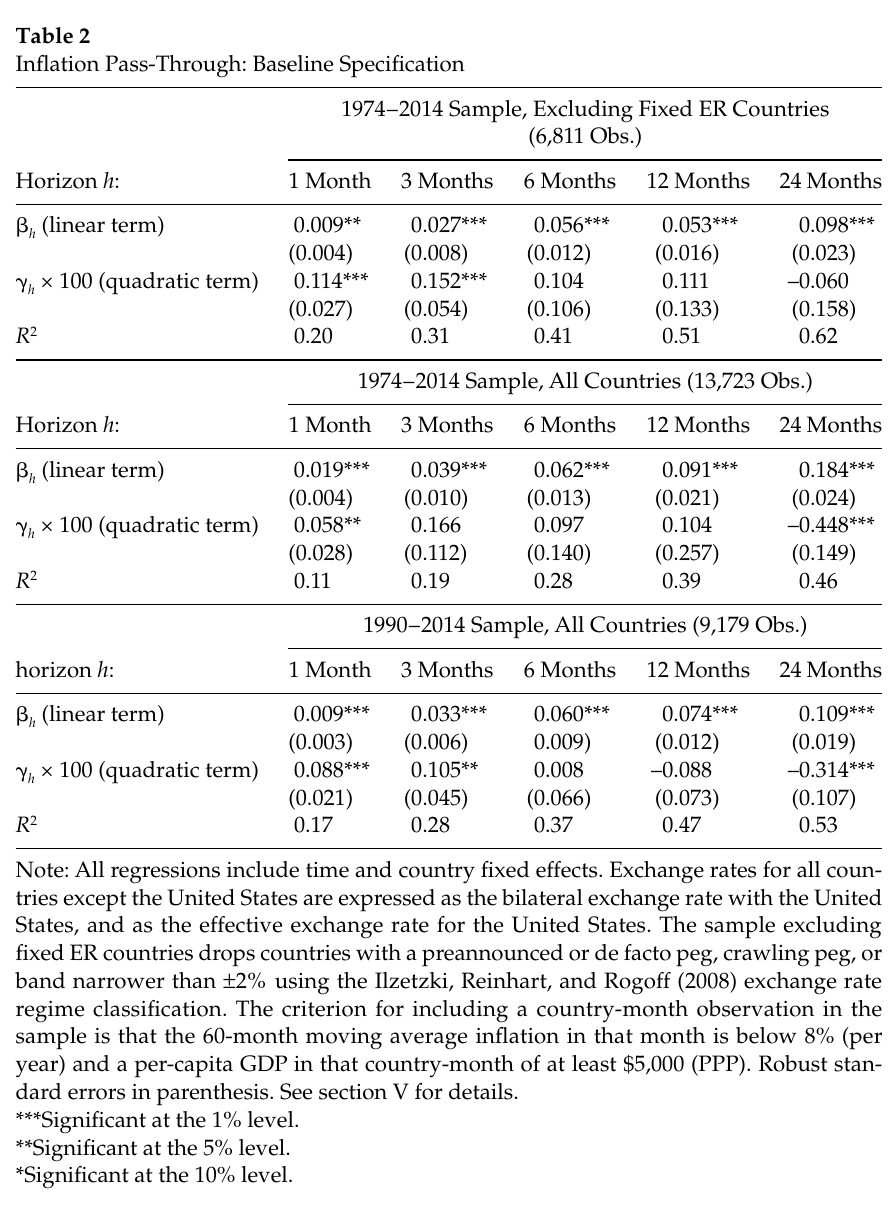
In the preferred no-peg panel (6,811 observations), the linear pass-through is 0.009 at one month and about 0.1 at two years. The quadratic coefficient, printed ×100, is 0.114 (s.e. 0.027) at one month and 0.152 at three months, and is insignificant from six months on. That is the shape sd predicts: big shocks pass through faster, and the difference has washed out by six months. In magnitude, a 10% devaluation adds about 0.2 percentage points to first-month inflation, roughly half of which comes from the quadratic term. In the talk Lippi said that at 10% the effect “basically doubles” relative to a small shock (00:16:48). That is the average response per unit of shock: $\beta + 10\gamma = 0.0204$ against about $0.0101$ at 1%. The introduction instead claims the elasticity at a 5.5% shock is “almost two times” the elasticity at 1%. That also checks out, but for the marginal response: $\beta + 2\gamma x$ gives 0.0215 against 0.0113, a ratio of 1.91. Both numbers are right; they measure different objects. The all-country panel keeps a significant one-month $\gamma$ (0.058), half the size, and the post-1990 panel gives 0.088. The robustness tables (a piecewise-linear kink at 10%, no time effects, dropping unclassified countries, the Levy-Yeyati–Sturzenegger (2003) classification) mostly keep the short-horizon result. Then there is Table 8.

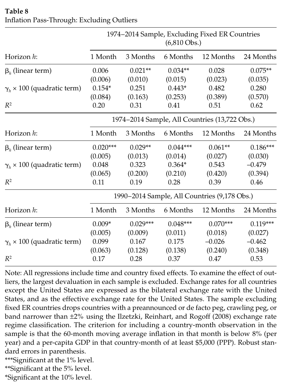
Drop the single largest devaluation in each sample, which in the preferred sample is a 46% Korean devaluation, and every panel loses 5% significance at one month. In the no-peg panel the one-month coefficient actually rises, to 0.154, but its standard error roughly triples, to 0.084. That leaves it significant at 10%, and the six-month coefficient is likewise significant at 10%. The all-country estimate slips from 0.058 to 0.048 and the post-1990 one moves from 0.088 to 0.099, neither significant. The authors report this up front, credit their discussant Greg Kaplan for raising it, and point out that the point estimates survive. The fair reading is a loss of precision, not a disappearance: a sample of low-inflation countries simply contains very few big devaluations (only five above 20% in the preferred sample, per p. 425), and one of them was doing most of the identifying.

What the talk adds

The talk gives about twelve minutes to the theory and five to the regressions, and it adds a few things. It gives the cleaner intuitions: the Calvo discretisation for td’s zero impact, and the red-triangle slide, which has no counterpart figure in the published chapter. It is franker about the empirics. In the captions’ rendering, Lippi called the empirical work “very preliminary” (00:19:32) and hoped it would prompt better tests. On identification he said there is “nothing deep about causations here”, that they are just running a regression and hoping the regressor is roughly orthogonal (00:14:43). It also states the policy reading the chapter leaves implicit: since policy exercises usually involve small shocks, the result is “reassuring for most applications” (00:19:04). In the other direction, the talk leaves out the Korea sensitivity, the threshold failures and the negative long-horizon coefficients. It also says “about 60” countries (00:13:59) where the chapter says about 70, and it notes that Ricardo Reis, one of the founders of the inattention view, was in the room (00:05:34). Talk quotations come from auto-generated captions and may be slightly off. The published volume also carries comments by the discussants, John Leahy and Greg Kaplan. Those are not covered here; the only traces in the chapter are two footnotes thanking Kaplan for the outlier point and for suggesting the no-time-effects specification.

Where it is soft (my reading)

The theory is clean within its stated scope, but the scope is real. Proposition 2 is local around zero inflation. It assumes continuous-path idiosyncratic shocks (so no Gertler–Leahy (2008) or Midrigan jumps), Golosov–Lucas general equilibrium with no strategic complementarities, and a quadratic profit approximation, and its analytic sd proof needs $\eta = \rho$. “Fit to the same kurtosis” is also not an innocent instruction, since the paper itself warns that measured kurtosis is sensitive to measurement error and heterogeneity. The td class also assumes firms cannot notice even a very large aggregate event before their scheduled review. Whether a model in which salient news triggers attention would still sit on the td side is a question the paper does not take up.

The empirics test the qualitative curvature prediction, not $\mathrm{Kurt}/N$. A bilateral dollar devaluation is not a common $\delta$ to every firm’s marginal cost; the paper treats it as a proxy. And a monthly cpi is averaged over the month, so the one-month response is not the instantaneous $\Theta$: even a discrete-time td model would show a first-month response, just a linear one. Large devaluations also cluster in crises and after real appreciations, which the authors acknowledge as an identification problem. Whether the Korean episode’s demand collapse biases pass-through up or down goes undiscussed, so treat that as an open question rather than a known bias. Other untested readings of $\gamma > 0$ include cross-country heterogeneity in pass-through that happens to correlate with shock size, invoicing currency, and state dependence at the importer rather than the retailer. Two patterns sit awkwardly with the theory. With a 4% inflation threshold, which the theory says should give the cleanest test, the nonlinearity is not significant (p. 422); the authors attribute this to there being fewer large devaluations. And the all-country samples give a significantly negative $\gamma$ at 24 months, which the authors candidly say none of the theories they review can fit.

Finally, there are small internal inconsistencies, none fatal. The text gives 13,025 observations for the main sample while Table 2 has 13,723. The inflation screen is described as a 10-year centred window in the text but a 60-month moving average in every table note. The paper says about 70 countries, but the appendix table lists 100 rows, including Bolivia, Burundi and Haiti, and how it maps to the regression panels is unclear. The Korean devaluation is dated 1996; the won crisis was late 1997, so this is probably a typo, though that is my guess. Std$(\Delta p)$ is given as $2\bar g$ on p. 409 and $\bar g$ on p. 415, and p. 415 is right. The p. 409 display also labels as $\Theta$ an expansion that the appendix derives for the fraction of adjusters, and prints a remainder weaker than the expansion supports. Prose on p. 415 says one standard deviation where eq. 32 says two. The text on p. 417 says inflation is slightly higher in the no-peg sample, while Table 1 shows it lower. And the summary claim that the result is not robust to adding pegs to the full sample is true only from three months on; at one month it survives.

None of this undoes the theory, which is the paper’s real contribution. A long-running argument about which friction is right turns out, for small shocks, to be an argument about two moments of the price-change distribution that both sides could have measured. The test meant to settle the large-shock case currently rests on very few large shocks, one of them Korean, and the authors are, to their credit, the first to say so.

References