Universal Gravity

Treb Allen (Dartmouth), Costas Arkolakis (Yale) and Yuta Takahashi (Hitotsubashi), “Universal Gravity,” Journal of Political Economy 128(2), 393–433, February 2020. This is the published version, read together with its online appendix. No talk recording was found, so this digest is written from the paper and the online appendix alone.

“Universal Gravity” is a paper about what quantitative trade and economic geography models have in common, and its answer is that, for most of the questions people actually ask them, they are the same model with two numbers. You pick Armington (1969), Krugman (1980), Eaton–Kortum (2002), Melitz (2003), or a spatial model where workers move and cities agglomerate. You spend a chapter of your dissertation on the microfoundations. Then you hand the model a matrix of observed trade flows and ask what happens if the us and China raise tariffs on each other. Allen, Arkolakis and Takahashi show that the answer for trade flows, incomes and real output prices depends on your microfoundations only through a demand elasticity $\phi$ and a supply elasticity $\psi$. Everything else was decoration, at least for the positive predictions.

That is the theory half. The empirical half is an attempt to estimate the two numbers directly, and the estimate of the supply elasticity comes out at about 68, which is where the paper gets interesting.

The model

The move is to throw away the micro model and keep only its aggregate shadow. Each of $N$ locations produces one representative good. Shipping it costs an iceberg wedge, $p_{ij} = p_i\tau_{ij}$, and some wedges may be infinite, so some pairs need not trade at all. Demand is ces with a constant elasticity, which delivers the gravity equation. Supply is also ces: location $i$’s output is $Q_i = \kappa\,\bar c_i\,(p_i/P_i)^{\psi}$, where $\bar c_i$ is an exogenous shifter and $\kappa$ a common endogenous scalar. Add goods-market clearing, exogenous deficits and a numeraire, and you are done. Under balanced trade the whole equilibrium collapses to $2N$ equations in output prices and price indices:

These are eqs. 6–7 in the paper, where $p_i$ is the output price, $P_i$ the ces price index, $\bar c_i$ the supply shifter and $\tau_{ij}$ the iceberg friction, so that $\phi$ and $\psi$ are the only parameters left. (With deficits each term on the right of the first equation picks up an expenditure-to-income factor and a world-clearing scalar; the price-index equation is unchanged.) Note that $\kappa$ appears nowhere. Trade flows, incomes and real output prices are pinned down; quantities, price levels and real expenditure are known only up to that scale.

Two notational traps. First, $\phi$ is the negative of the demand elasticity, so $\phi \ge 0$ means demand slopes down; in Armington it is $\sigma - 1$, in Eaton–Kortum it is $\theta$. Second, $\psi$ is an elasticity of aggregate output with respect to the real output price $p_i/P_i$. It is not a claim that labor supply has elasticity $\psi$, and it does not care where it came from.

Which is the clever part, because the obvious objection is that trade models have fixed labor and should therefore have $\psi = 0$. They don’t, once there are intermediate inputs. You hold labor fixed. Your output price rises relative to the price index, and the price index is also the price of your intermediates. So you buy more intermediates and produce more gross output. With a Cobb–Douglas (1928) labor share $\zeta$ in a roundabout technology, $\psi = (1-\zeta)/\zeta$. In the Allen–Arkolakis (2014) geography model the same exponent comes from people moving toward high real wages, with $\psi = -(1+a)/(a+b)$ in terms of the productivity and amenity spillovers $a$ and $b$; with $a > -1$ it is positive only when dispersion forces win. The aggregate equations cannot tell these two stories apart, and the paper is happy about that. The celebrated Arkolakis–Costinot–Rodríguez-Clare (2012) class is the special case $\psi = 0$.

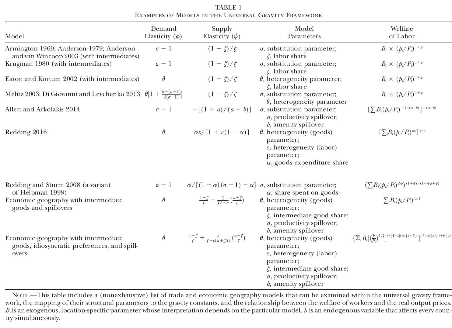
Table 1 is the paper’s dictionary. Read across a row and you get that model’s $\phi$ and $\psi$ (the Melitz row is not simply $\phi = \theta$, for the record). Read the last column and you see the honest limit of the whole exercise: the map from real output prices to welfare differs model by model. So the positive predictions are universal and the normative ones are not, which the authors say plainly in a footnote. What is outside the tent is also stated: non-constant elasticities, multiple sectors, multiple factors with varying intensities, endogenous deficits. Tariff revenue gets a worked Armington example in the online appendix, not a universal equivalence.

When the equilibrium exists and is unique

Theorem 1 gives conditions on $(\phi, \psi)$ alone, assuming balanced trade, finite domestic frictions and a strongly connected graph of finite trade links. An interior equilibrium exists if $1 + \phi + \psi \neq 0$. All equilibria are interior if $\phi \ge -1$ and $\psi \ge 0$. The interior equilibrium is unique if both elasticities are nonnegative, or both are at most $-1$; with quasi-symmetric frictions the bounds relax to $-1/2$. Every one of these is a sufficient condition, and the paper is careful to say so. On the line $1+\phi+\psi = 0$ existence may fail, and the examples are Leontief Armington and the economic-geography black hole, where agglomeration is exactly strong enough to pull everyone into one place.

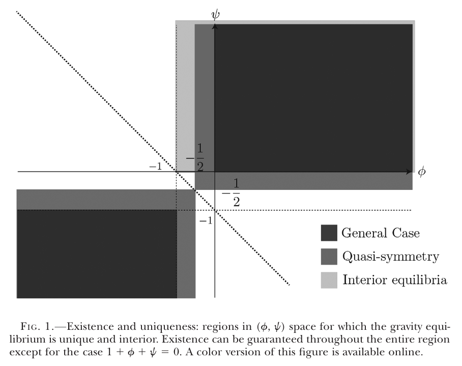
The intuition is the textbook one with the textbook’s sign convention restored: uniqueness when demand slopes down and supply slopes up. Multiplicity examples appear when the two slope the same way, as with complementary goods in a trade model or strong agglomeration in a geography model. The proof rewrites the system as nonlinear integral equations and extends a Karlin–Nirenberg (1967) max/min-ratio argument to systems. A small payoff relative to Alvarez and Lucas (2007): gross substitutes is guaranteed when $\phi > \psi > 0$ but can fail when $\psi > \phi \ge 0$, and the paper’s own estimates land in exactly that second region, where Theorem 1’s parameter inequalities still hold. That covers the parameter half of the theorem; the balanced-trade hypothesis is a separate matter, to which we return.

Counterfactuals as a matrix inverse

Theorem 2 is the practical result. Totally differentiate the deficit-inclusive system and you get $(S - D)\,d(\ln p, \ln P) = T\,d\ln\tau$, where the supply matrix $S$, the demand matrix $D$ and $T$ are built from $\phi$, $\psi$ and observed trade flows, incomes and expenditures, and nothing else. Provided the observed trade matrix is strongly connected and the system has the right rank, one (pseudo)inverse gives the elasticity of every country’s output price and price index to every bilateral friction (eq. 18 in the paper). So conditional on $(\phi, \psi)$ and the data, local counterfactuals for real output prices, trade flows and incomes are identical across every nested model. Deficits are allowed here, and the elasticities are valid around the observed equilibrium even if other equilibria exist.

If the spectral radius of $S^{-1}D$ is below one, the inverse expands as a series, and each term has a reading: shift demand, let the hit location re-equilibrate along its own supply curve, pass the change to its partners, then to its partners’ partners. This is the network-propagation logic familiar from production networks (see the reading note on Baqaee and Farhi), here running through the trade graph instead of the input–output graph. With quasi-symmetric frictions, balanced trade and nonnegative elasticities, the authors also prove that the directly hit pair suffers more than any bystander, which is reassuring and not exportable to asymmetric or deficit economies.

Estimating the two numbers

Anyway: if the whole thing is two numbers, you had better know them, and the paper shows that data alone never will. For any $(\phi, \psi)$ and any unobserved shifters there exists a unique set of off-diagonal frictions that rationalises the observed trade matrix exactly. You need an identifying restriction.

The procedure has two steps. First, run a gravity regression of $\ln(X_{ij}/X_{jj})$ on 360 dummies (ten distance deciles crossed with origin and destination continents) plus origin and destination country effects. Second, regress the recovered country effect on income and the own-expenditure share:

This is eq. 22 in the paper, where $\hat\pi_i$ is country $i$’s estimated effect from the first step, $Y_i$ its income, $\lambda_{ii}$ the share of its spending on its own goods, and $\nu_i$ collects the unobserved supply shifter, the domestic friction and estimation error. The problem is that $\nu_i$ is an equilibrium object’s cousin: productive places are rich and buy a lot from themselves, so ols is biased, and $\phi$ biased down in particular.

The fix is a “model-implied” instrument. Solve the model in a hypothetical world where frictions come only from the fitted distance-and-continent profile and supply shifters are either equal across countries or predicted from observables. The hypothetical income and own share become instruments for the real ones, with the observables also entering as controls, so the identifying variation is purely the general-equilibrium effect of geography: being near big markets and having big neighbours. The exclusion restriction is that geography is uncorrelated with the unobserved shifters conditional on the controls. Solving a model does not make that true; a set of remote countries that are also intrinsically unproductive for reasons the controls miss would break it.

One elegant wrinkle. The workhorse assumption that makes uniqueness easier, quasi-symmetric frictions, kills identification here: under quasi-symmetry and balanced trade the hypothetical income and own share are log-linearly related, so the instruments are collinear. The paper deliberately uses directed continent-pair distance effects to break the symmetry. The asymmetry in the gravity fit is doing identification work, not just improving the fit.

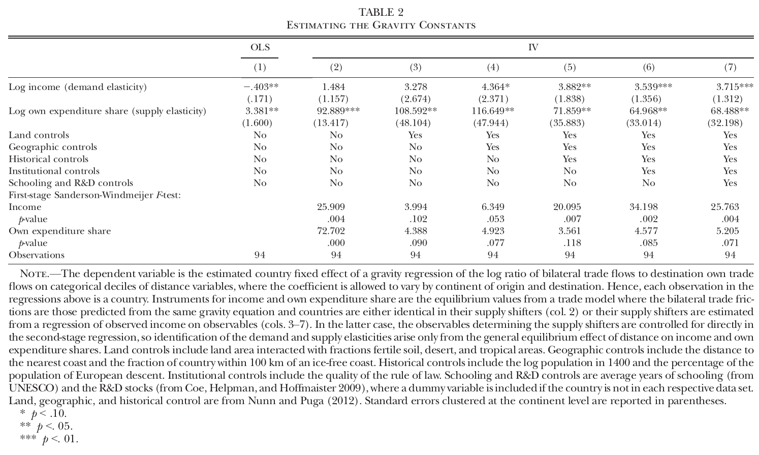
The data are gtap for 2004, 94 countries. ols in column 1 gives $\phi = -0.403$: demand sloping the wrong way, which is what the predicted bias looks like when it wins. The iv columns add controls in stages (land, geography, history, institutions, schooling and R&D), and the preferred column 7 gives $\phi = 3.72$, with a 95% interval of $[1.14, 6.29]$, and $\psi = 68.49$, with an interval of $[5.38, 131.60]$. The demand elasticity sits comfortably with the literature’s values around 4 and below Eaton–Kortum’s preferred 8.28. The supply elasticity is, in the authors’ phrase, “substantially larger” than the 3.76 implicit in Eaton–Kortum’s calibration, and statistically different from it at 5%. The authors flag themselves that the own-share first stage is only marginally significant, so some of that width may be a weak instrument.

The one surprising thing: $\psi \approx 68$

Take 68 seriously and run it back through Table 1. In the trade-with-intermediates reading, $\psi = (1-\zeta)/\zeta$ means a labor share of gross output of about 1.4% (our arithmetic; the confidence interval’s endpoints give roughly 16% and 0.75%). Nobody believes that. In the Allen–Arkolakis reading with $a = 0.10$, $a + b \approx -0.016$ (our arithmetic again): dispersion forces barely beating agglomeration. That is not the black-hole line where existence fails, which at these estimates is far away ($1+\phi+\psi \approx 73$). It is close to $a + b = 0$, where $\psi$ flips from $+\infty$ to $-\infty$ and the economy would leave Theorem 1’s sufficient region for uniqueness. That is only suggestive, since sufficient conditions are silent about what happens once you cross them.

The authors choose a third reading for interpretation: in a geography model with intermediates, agglomeration and Fréchet location preferences, $\psi = 68.49$ is “consistent with” a migration elasticity of 1.4, between a third and a half of within-country estimates. That makes 68 sound plausible. (A small reproducibility note: plugging the stated labor share 0.21 and $a = 0.10$ into Table 1’s last-row formula with no amenity spillover gives about 1.7, not 1.4; getting 1.4 seems to require an amenity spillover the text does not state. It doesn’t matter for anything else, but the number is not reproducible from the page.) So the paper interprets $\psi$ through migration, and as we will see it computes welfare-like numbers through the Armington reading, where 68 means a 1.4% labor share.

The trade war

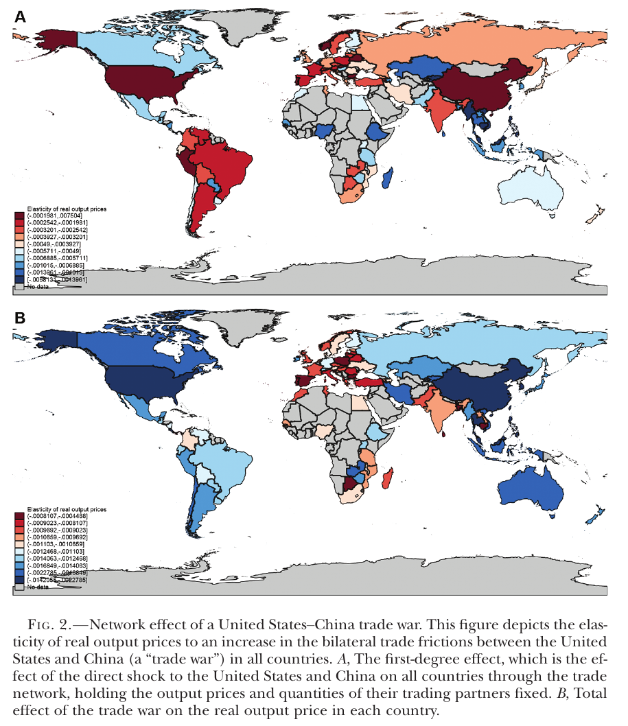
The application raises us–China frictions in both directions, holds every other friction and the observed deficit ratios fixed, and uses Theorem 2’s local elasticities on 2004 data. It is a model counterfactual, not evidence about the trade war that later happened. Because deficits are kept, Theorem 1’s uniqueness result, which is stated for balanced trade, does not formally cover this economy; what licenses the exercise is Theorem 2’s local result around the observed equilibrium, given connectivity and the rank condition. The degree-by-degree decomposition is the nice part. At degree zero both countries export less, so their output prices fall, and import prices rise, so their price indices rise. At degree one something counterintuitive appears (panel A): the us and China gain, because their own cheaper output lowers their own price indices, while their big trading partners lose. The total effect (panel B) is negative everywhere, worst in the us and China, and worse in tightly connected partners such as Canada, Mexico, Vietnam and Japan than in less-connected India.

Now the magnitudes. A 10% rise in bilateral frictions lowers the real output price by 0.04% in the us and 0.14% in China. Those are tiny, and the reason is the large $\psi$: output reallocates away rather than prices falling. The converse, in the authors’ Armington interpretation, is that real expenditure falls by 2.7% in the us and 9.8% in China. These two sets of numbers are the same result. Real expenditure is proportional to $(p_i/P_i)^{1+\psi}$, so the second set is the first multiplied by 69.49 (69.49 × 0.04 ≈ 2.8, 69.49 × 0.142 ≈ 9.9). The paper’s headline, “modest declines in (real) prices but large declines in (real) expenditure,” is one estimate read twice. A global 50% shock solved by exact hat algebra lines up with the local elasticities (correlation above 0.99), with magnitudes about 80% as large. For other readings of the us–China episode built on actual tariff data, see the notes on The Return to Protectionism and the economic impacts of the us–China trade war.

What a discussant might push on (our note, not from any talk)

Standard errors are clustered by continent, which means six clusters. The reported first-stage p-values match an F(1,5) reference, but the confidence intervals use ±1.96. With the t(5) critical value of 2.571, the $\psi$ interval runs from about −14 to about 151 (our arithmetic). The “different from 3.76 at 5%” claim, which rests on a t-statistic of about 2.01, would not survive, and the interval would cross into $\psi < 0$, outside the general uniqueness region. Add the marginal own-share first stage and the untestable exclusion restriction, and the real-expenditure numbers become the paper’s least settled output. They carry a $1 + \psi$ multiplier that ranges from about 6 to about 133 across the reported interval. But the price response they multiply also shrinks as $\psi$ grows, and the paper reports sensitivity over the $(\phi, \psi)$ box only for real output prices (us −0.03% to −0.05%, China −0.07% to −0.26% per 10%). Whether the expenditure numbers are more or less stable than the price numbers would take a joint recalculation, which nobody has shown.

None of this dents the theory, which is the durable contribution: a referee can now ask any spatial model what its $\phi$ and $\psi$ are, and most of the model’s positive behaviour follows. The paper’s own estimate just suggests that the second number is either very large or very hard to pin down, and the elegant part was showing that it was the only one left to pin down.

References