Does Foreign Direct Investment Promote Growth? Exploring the Role of Financial Markets on Linkages

Laura Alfaro (Harvard Business School), Areendam Chanda (Louisiana State), Sebnem Kalemli-Ozcan (Houston) and Selin Sayek (Bilkent), “Does foreign direct investment promote growth? Exploring the role of financial markets on linkages,” Journal of Development Economics 91(2), March 2010, 242–256. Written from the published version. There was no talk, and so no discussant.

The literature this paper is built to explain has an awkward shape. Ask whether a domestic firm in a poor country gets more productive when multinationals enter its own industry, and firm-level panels say no, and fairly often worse than no. Ask whether it gets more productive when it sells to one, and the answer turns positive — Javorcik on Lithuania, Alfaro and Rodriguez-Clare on Venezuela, Chile and Brazil. Ask at the country level whether FDI raises growth and you get “it depends,” with the dependence loading onto human capital (Borensztein, De Gregorio and Lee) or onto financial development (these authors’ own 2004 paper). Any theory that explains one of those facts tends to embarrass the other two.

So the authors write down the model in which the multinational transfers no technology whatsoever. Not a little, none. The foreign process is more productive than the domestic one — twice as productive, in the benchmark — and more skill-intensive, and that advantage stays sealed inside the firm forever; nothing leaks, nobody imitates, no engineer quits and starts a competitor. What the multinational does instead is buy things. It buys the same non-traded differentiated intermediate inputs, from the same local monopolistically competitive suppliers, spending the same share of revenue on them as a domestic firm would. Foreign entry is therefore, mechanically and only, a demand shock to the local supplier sector. The multinational is not a teacher. It is a customer.

The model

You are an entrepreneur in this economy with an idea for a new variety of intermediate input. To bring it to market you must sink a fixed startup cost, $K = a(L+H)/n^{\theta}$ (eq. 21, p. 246) — capital only, scaled by the labor force so there are no scale effects, and falling in the varieties already invented, because you stand on shoulders. You cannot self-finance. You borrow the whole thing from the domestic financial system, which charges you $i$ while the world lends at $r$, and free entry drives you to the point where the present value of your interest payments equals the value of the firm you have created (eq. 22, p. 247). The wedge $i - r$ is what “financial development” means in this paper: not rationing, not collateral, not wealth — a spread.

Two equations carry the argument. The first defines foreign presence:

$Y_{t,d}$ and $Y_{t,f}$ are the domestic and MNE processes’ output, $\mu$ is the weight on the foreign one, and $\varepsilon = 1/(1-\rho)$ is the elasticity of substitution between them (eq. 3, p. 244). The authors are candid that this is “an artifact”: they do not model the multinational’s decision to enter, so $\mu$ is simply a dial they turn. The second is the balanced growth rate of varieties:

The bracket is efficiency-adjusted downstream output value per worker; $\lambda$ converts it into intermediate spending and $1-\alpha$ is the markup share of that spending which accrues to variety producers as profit (eq. 30, p. 247). So the bracket is the market, and $i$ sits in the denominator. Turn up $\mu$, expenditure shifts toward the more productive process, the market for local inputs gets bigger, entry accelerates, $n$ rises, and the variety externality lifts total factor productivity in both downstream processes — the backward linkage arriving, one lag later, as a horizontal spillover. And the identical push buys less entry wherever intermediation is expensive. That is the whole interaction, and it is entirely pecuniary.

It also explains the negative micro spillovers rather than apologizing for them. The instantaneous effect of more foreign presence is reallocation away from domestic firms; the productivity gain accrues only to the survivors, and only as varieties accumulate. A panel of incumbents can record zero or negative horizontal spillovers while the aggregate growth effect is positive.

The numbers, and which experiment they come from

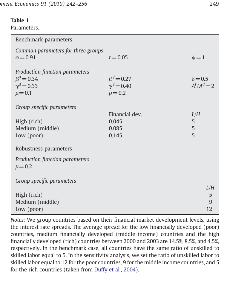
Almost nothing here is estimated. The intermediate share $\lambda = 1/3$ comes from Gollin, the markup from Basu, the productivity gap $A_f/A_d = 2$ from Hall and Jones, the elasticity $\rho = 0.2$ from Ruhl’s reading of the Armington literature, the unskilled share in variety production $\delta = 0.5$ from nowhere at all (“given the lack of any estimate,” p. 249), and $\theta \approx 0.967$ from the requirement that sectoral output and GDP grow at the same rate. Exactly one parameter is fitted: $a = 0.6$, set so the financially developed group grows at the U.S. rate of about 3.5%, assuming the U.S. has no foreign productivity advantage to speak of. The dial $\mu = 0.1$ is not an input read off anything but a setting chosen to hit a target — it makes the model’s foreign output share 6.1%, against Lipsey’s estimate that FDI was at most 8% of world production. And the three spreads — 4.5%, 8.5%, 14.5%, group averages for 2000–03 — are measured, and are the only thing distinguishing rich from poor in the benchmark.

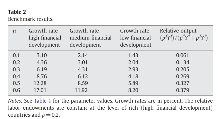
Which means the level results are pure out-of-sample predictions from three interest-rate spreads. At $\mu = 0.1$ the model gives 3.10% growth under high financial development, 2.14% under medium and 1.43% under low. Identical foreign presence, identical everything else, more than double the growth. (The paper does not check these against the groups’ actual growth rates.)

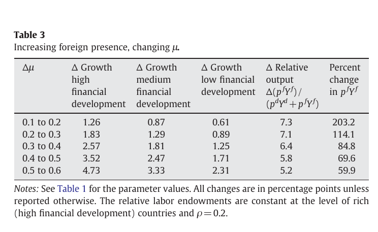
Then two different experiments, which it is worth keeping strictly apart. Turning the dial $\mu$ from 0.1 to 0.2 — the foreign output share rises 7.3 points, foreign output triples — adds 1.26 percentage points of growth in the rich group against 0.61 in the poor one. The authors volunteer that 1.26 is probably an overestimate: a twofold productivity gap is too wide for a rich host, and later foreign entrants are likely less productive than the first ones (p. 250).

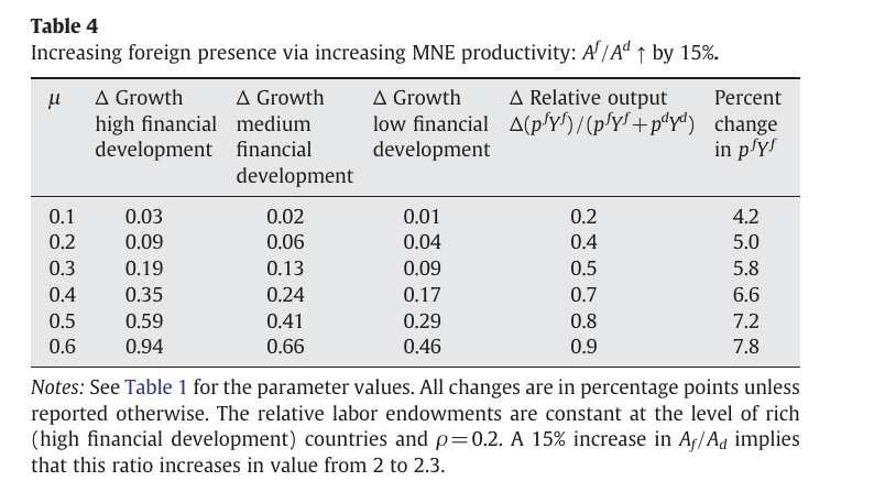
The other experiment upgrades the multinational instead: raise $A_f/A_d$ by 15%, from 2 to 2.3, holding $\mu$ fixed. That adds 0.03 percentage points for the rich group, 0.01 for the poor. Comparing the first rows of the two tables gives ratios of roughly forty for the developed groups and sixty for the poorest — my arithmetic, not the paper’s, which says only “quantitatively much lower” and warns that the two shocks “may not be strictly comparable.” The resolution is that raising $\mu$ shifts expenditure toward the productive process by construction, while raising $A_f$ has to work through relative prices, and at $\varepsilon = 1.25$ the induced share shift is 0.2 of a percentage point. Normalize by that and the two experiments nearly agree: per point of MNE output share, growth rises 0.17 versus 0.15 in rich countries, 0.08 versus 0.05 in poor ones (p. 251). Which is a quietly useful lesson about what cross-country FDI regressions are measuring — not FDI, but the share of output it happens to occupy.

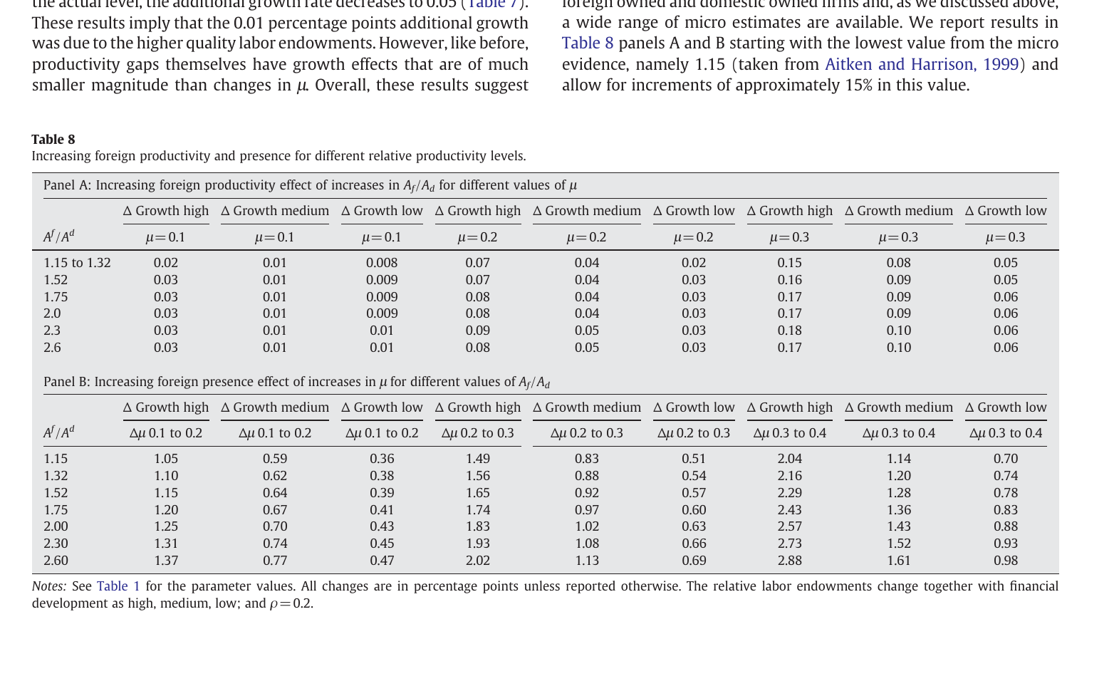
The financial-development ordering survives everything the authors throw at it. Vary the productivity gap across the whole micro-to-macro range and the $\mu$-experiment increments barely move. Let the poor group have its true unskilled-heavy endowment instead of the rich group’s and its growth falls further, so that human capital compounds the finance channel — “three times more” rather than twice, in the paper’s own words (p. 251).

The trap

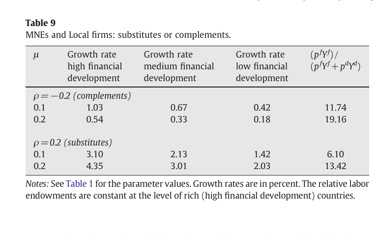
Everything above is signed at $\rho = 0.2$, domestic and foreign output substitutes. Set $\rho = -0.2$ and make them complements, and raising the FDI share cuts growth — the financially developed economy goes from 1.03% to 0.54% while the multinationals’ share of output rises from 11.74% to 19.16%. More FDI, more foreign output, less growth. The algebra is not mysterious once you look at the aggregator: with $\rho < 0$ the outer exponent $1/\rho$ is negative, so a larger $\mu$ lowers final output for given sectoral outputs, which shrinks the market local suppliers sell into, which is the only thing in the growth equation that FDI can move. (Only the $\mu$ dial flips. Upgrading the multinational still buys small positive increments under complements.) The paper’s own gloss is thinner than that — “the elasticity of substitution in the aggregator plays a key role” — but it draws the right moral, which is the best line in the paper: “one must be cautious when talking of attracting ‘FDI that is complementary to local production.’ Such complementarity is useful when one talks of final and intermediate industry relationships. However, it does not necessarily raise the growth rates when domestic and foreign producers supply complementary final goods” (p. 253). The complementarity you want is vertical. The complementarity in the investment-promotion brochure is horizontal, and in this model it is a tax.

What a reader should push back on

The objections write themselves, and to its credit the paper hands you most of the ammunition. The whole thing is signed by an elasticity borrowed from an unpublished survey of an Armington literature whose estimates are famously all over the place, and flipping it flips the sign of the headline result. “Financial development” is a spread between groups labeled rich and poor, and since anything that raises the entrepreneur’s cost of borrowing enters the model identically — a footnote of the authors’ own lists taxes, reserve requirements and administrative costs among the sources of the wedge — the exercise cannot separate finance from the general cost of doing business locally. FDI is exogenous twice over, with no entry decision and no channel by which good financial markets attract foreign firms, which is the obvious alternative reading of the very correlation the model is rationalizing; the conclusion concedes as much. The best micro support for the mechanism, Javorcik and Spatareanu’s finding that Czech suppliers to multinationals are less credit constrained, is something the authors themselves report as self-selection. The engine is a TFP elasticity to variety of about 0.033, so assuming a 20% markup instead of 10% roughly doubles it. And a permanent 1.26-point growth gain from a one-time move in the FDI share is an enormous object to hand a policymaker — though that is an outside-the-model complaint, since inside the model the growth rate is genuinely permanent and genuinely policy-dependent.

One inconsistency is worth flagging because the paper cannot be right both times: the text under equation (3) says Cobb–Douglas is $\varepsilon = 1$, which is the $\rho \to 0$ limit, while footnote 38 on p. 253 calls $\rho = 1$ “the Cobb Douglas case,” which in that aggregator is the linear, perfect-substitutes case. The Cobb–Douglas solutions live in an appendix available on request, so you cannot check which one the numbers used.

Still, the thing the model buys is real, and it is not the calibration. It is that you can generate the entire macro FDI-and-growth literature — conditional effects, absorptive capacity, the financial-development interaction — out of a multinational that teaches nobody anything and merely places orders. Everyone has spent thirty years looking for the knowledge that spills over. The paper’s answer is that the spillover may just be the purchase order, and that whether it turns into anything depends on what your local suppliers are charged to borrow.