Artificial Intelligence and Labor Market Reallocation

Start with what an unemployment rate is, because the entire disagreement in this literature lives there and nowhere else. A group’s unemployment rate is not a measurement of how much trouble that group is in. It is the slow accumulation of two fast flows — the rate at which the employed separate and the rate at which the unemployed find work — and in steady state it is just the ratio of the first to their sum. Which means it is possible for a group’s hiring to fall off a cliff while its unemployment rate does something that looks, for a year or two, like nothing.

Illustrate it on the back of an envelope. Take a group where 0.8% of the employed lose their job in a given month and a quarter of the unemployed find one; that is a steady-state unemployment rate a shade over 3%. Now cut job-finding by a fifth and leave separations exactly where they were. The new steady state is about 3.9%, and the path there takes the better part of two years, most of which is indistinguishable from noise. Nobody was fired. Something quite large happened anyway.

This is why the ai-and-jobs literature has mostly been reading the wrong object. It reads stocks — employment and unemployment by occupation — and finds, as The Budget Lab at Yale did in 2025, effects that are small or negligible. A stock is a lagging integral of the thing you wanted to measure. Hie Joo Ahn and Nicholas Carollo of the Federal Reserve Board went and built the flows instead, by ai exposure and by ai adoption, and then ran the standard natural-rate machinery over the pieces. Ahn presented it on the first afternoon; it is a 92-page conference draft dated September 2026, unpublished, preliminary enough that two of its cross-references still print as an unresolved “??”, and it carries the usual line that nothing in it is the view of the Board. Carollo, she said, was in the room “to answer difficult questions.” When the chair turned to him at the end he declined to have any.

The two scores, and the asymmetry between them. Exposure is the Eloundou et al. (2023) measure: the fraction of an occupation’s O*net tasks that an llm plus complementary software could do at at least 50% time saving without loss of quality, assigned by gpt-4, weighted up to eight-digit occupations with supplemental tasks counted at half the weight of core ones. It varies by occupation and not by time — it is a statement about what the technology can do, which Ahn reads as the supply side, “ai’s feasibility of conducting human tasks.” Adoption is the share of Lightcast job postings in a three-digit industry carrying a skill tag whose description mentions artificial intelligence or machine learning. It varies by industry and by month, and Ahn reads it as the demand side, “actual labor demand for ai-integrated roles for production.” It correlates robustly and positively with the Census Bureau’s btos firm-level ai-use question at the three-digit naics level, which is about as much external validation as exists. The paper also lists its own measurement worries without being asked: postings miss ai that incumbents are already using, and a boilerplate disclaimer that a firm may use ai tools in hiring gets tagged as adoption.

Both scores then get attached to cps respondents, which is easy for the employed and awkward for the unemployed. The unemployed report a previous industry and occupation, but about 10% either have none or report a military occupation with no score, so there is a four-rung imputation ladder that ends, for people with no work history at all, at the mean of demographically similar people who worked exactly one month in the panel — a deliberate proxy for weak attachment. The third rung is the baseline and leaves 5% unscored. The honest footnote is that people with missing ai scores account for about 0.2 pp of the 0.7 pp rise in the aggregate unemployment rate over the period, which is not nothing, and that under full imputation the bottom exposure group’s rise doubles from 0.4 pp to 0.9 pp — still below the top group’s, but the gap narrows. Vacancies, needed for tightness, come from splitting jolts industry openings across occupations by Lightcast posting shares, which forces the occupational series to add up exactly to jolts.

Now the part where the whole result is made, which is the bins. Exposure is cut at fixed task-share cutpoints — below 25%, 25–50, 50–75, 75 and above — and not at employment-weighted quartiles. Ahn flagged this on the slide and again out loud: “note that this is not the quartile concept, for example the labor force share of the top exposure group is only 4 percent.” Roughly twenty occupations, 4% of the labour force: software developers, computer programmers, accounting and auditing clerks. Adoption is cut at the 25th, 50th and 90th percentiles, because adoption varies continuously across industries with no natural breakpoints, and the object of interest is the top decile. The paper is not coy about what this buys: “we focus on workers at the right tail of the ai exposure and adoption distribution — the top 5th and 10th percentiles … Studies that rely on coarser groupings, such as quartiles, are unlikely to detect effects concentrated at the tail.” A footnote goes further and says that if you cut adoption into plain quartiles instead, “this pattern is masked.” That footnote is simultaneously the explanation of why this paper finds something everyone else missed and the reason to keep one hand on your wallet, and both readings are true at once: a real effect concentrated in a few percent of the labour force is exactly the kind of thing coarse bins destroy, and a specification chosen to make a tail visible is exactly the kind of thing that makes tails visible.

The levels, before any of the changes. Read this table first, because it is the setup for everything and it is the opposite of what you expect.

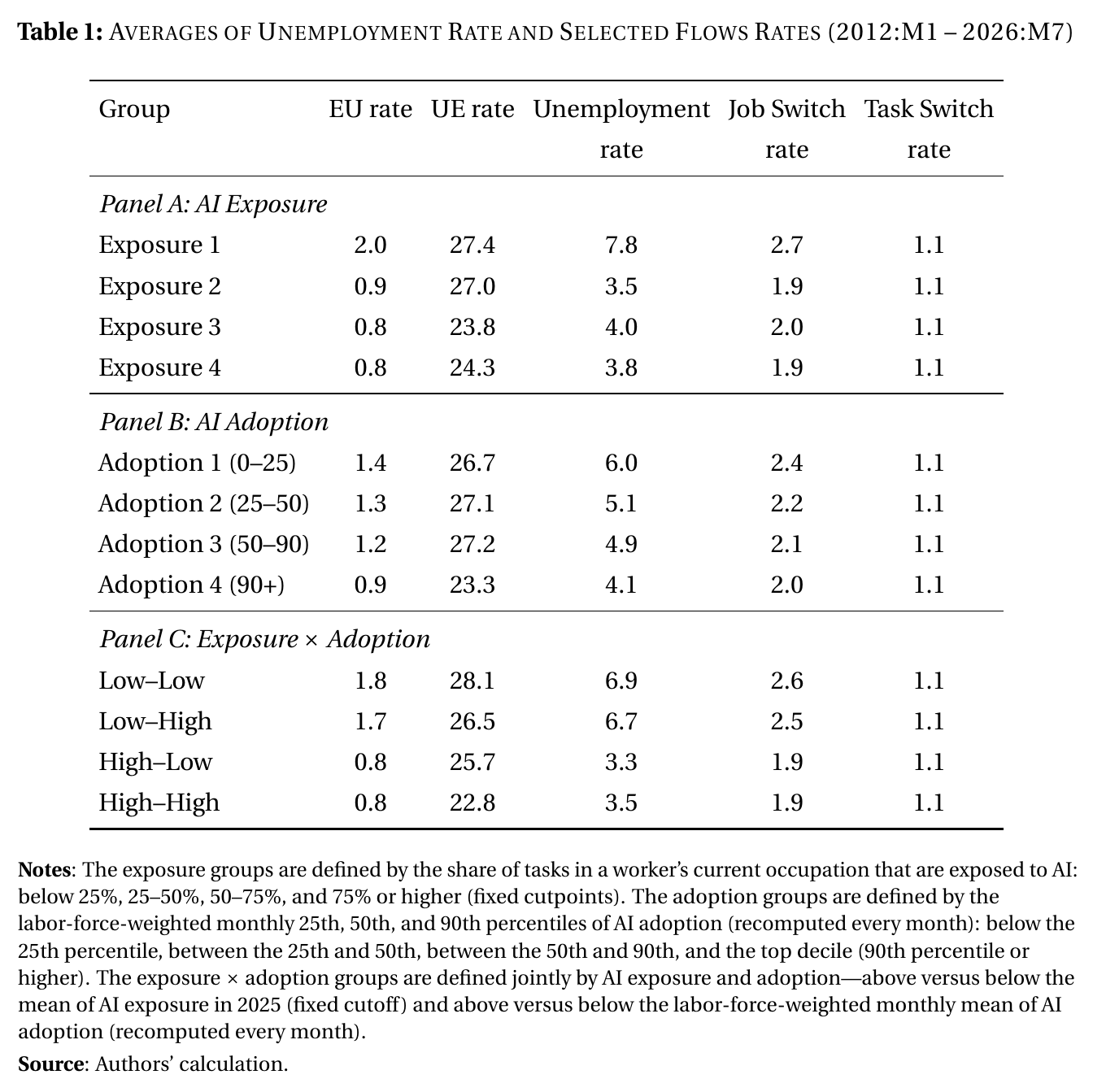
Workers with both high exposure and high adoption have the lowest unemployment rate in the economy, 3.5% against 6.9% for the low-low group. They have the lowest separation rate, 0.8 against 1.8. And, because none of this comes free, they have the lowest job-finding rate too, 22.8 against 28.1. Software developers and lawyers in legal services are not a fragile population. They are the most structurally insulated workers on the chart.

Which is precisely why the next picture counts for more than it looks like it does.

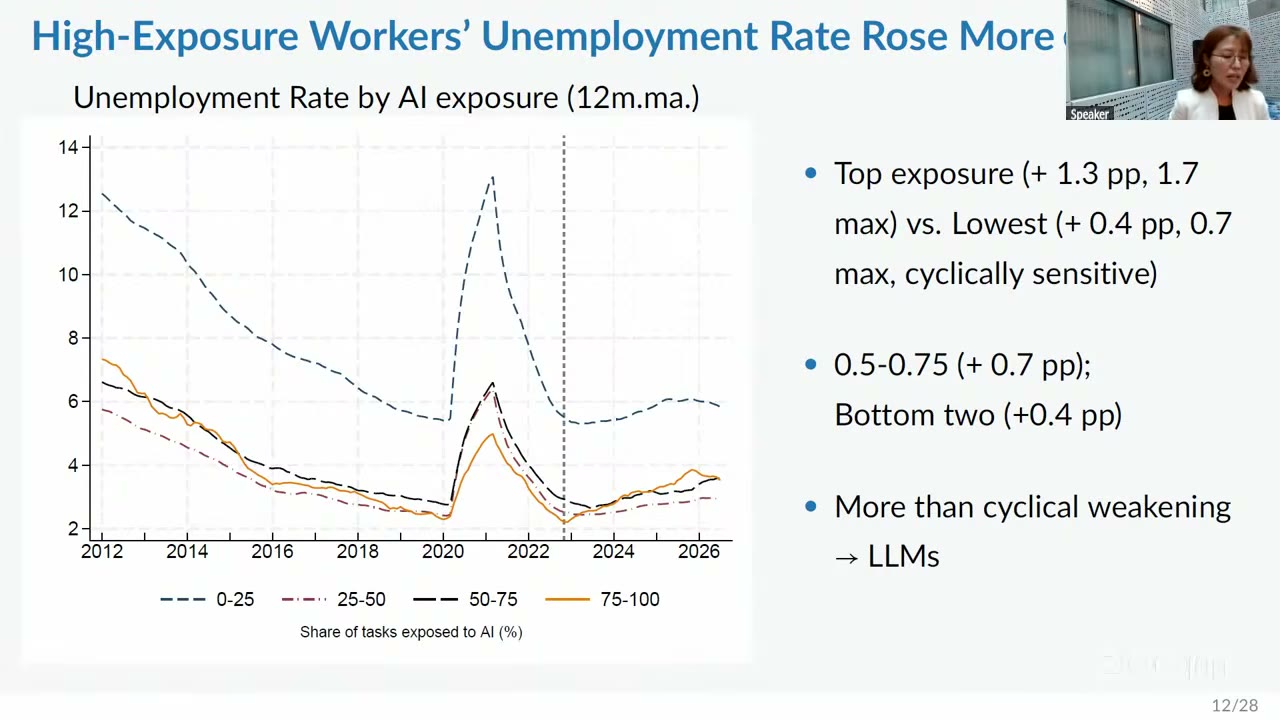
From the end of 2022 through July 2026 the top exposure bin’s unemployment rate is up 1.3 pp, and was up 1.7 pp at its late-2025 peak. The bottom bin is up 0.4 pp, and 0.7 pp at its own peak. The two middle bins land between. The top decile of adoption is up 1.2 pp against 0.4 pp for the bottom quartile. On the joint cut, high-exposure/high-adoption is up “slightly below 1 percentage point” and high-exposure/low-adoption about half a point, and Ahn’s reading of the difference between those two is the cleanest statement of what adoption is doing in this paper: “the gap actually reflects the effect of the adoption.”

The identification argument is the inversion. Normally in macro you want the treated group to move a lot. Here the treated group is the one whose unemployment rate barely moves at all — the flattest line on a chart where the untreated line swings seven points across a cycle and thirteen in 2020. Ahn: “Considering that this top exposure group’s unemployment rate is least cyclically sensitive, the fact that its unemployment rose more than the bottom group actually means that it reflects more than cyclical, and hence likely to reflect large language models’ effects.” The draft says the same thing more flatly: the faster rise among high-exposure workers “therefore likely reflects factors specific to them — above all, the introduction of llms.” It is a genuinely unusual position to be in. The evidence is strong because the affected population is small, well-paid and normally recession-proof.

And the adjustment is entirely on the hiring margin. Job-finding rates fall for the exposed groups and stay low. Separation rates for the top-exposure and high-high groups did edge up in 2025–26, but the differences across groups remain small, and in the regressions every high-ai group is less likely to be separated than the low-low baseline. Job-to-job transitions, which are the other hiring margin, fall too, and did not join the recovery that other groups’ switching rates began in the second half of 2025. Meanwhile, within-job activity switching — the cps asks whether your duties changed even though your employer didn’t — rises from around 2025, and rises fastest for exactly the groups where the hiring fell.

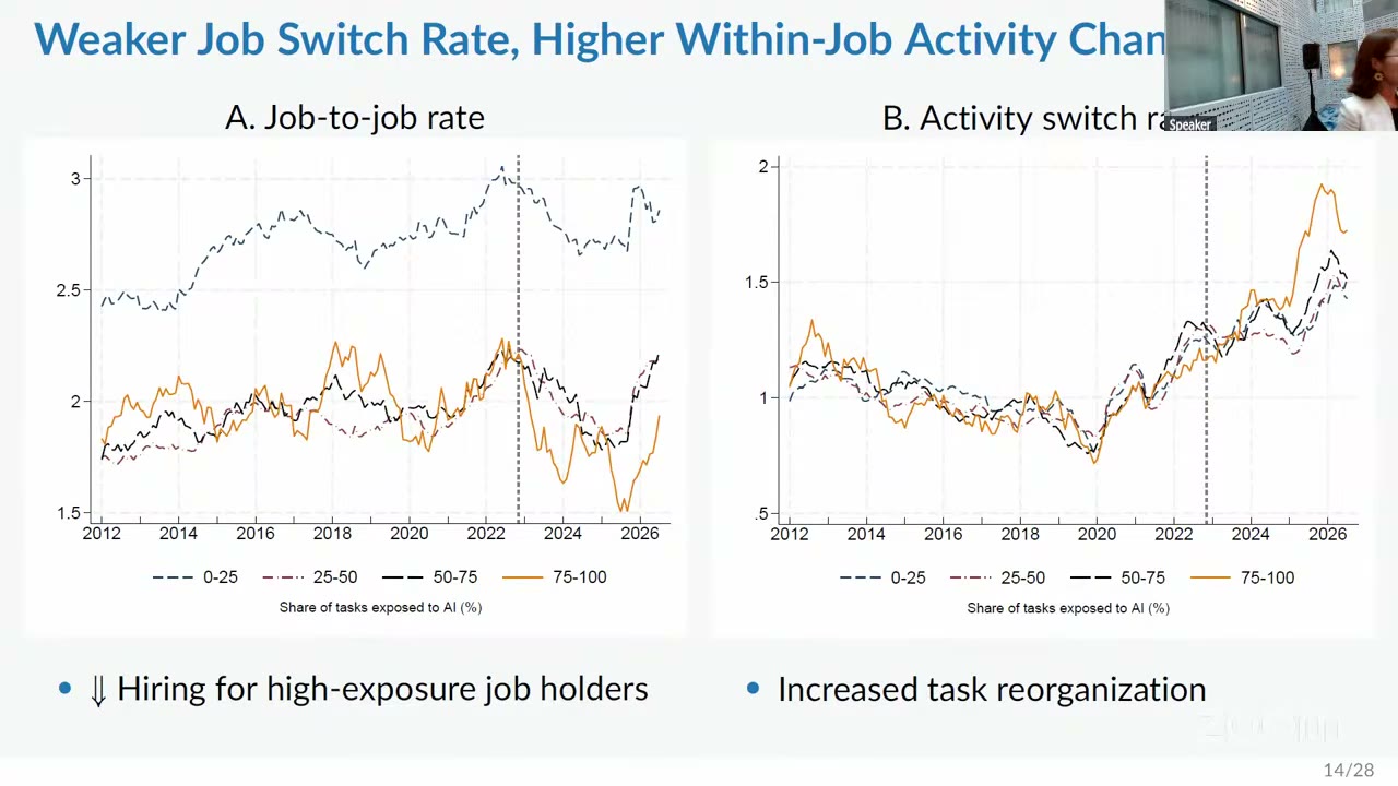
Put those together and the shape of the thing is: don’t hire, reorganise. Firms with ai in the building are not emptying desks; they are rearranging what the person at the desk does, and not opening the next req. That distinction is not a softening. It is the actual finding, and it is what the separation evidence licenses. Every sentence in this piece that could have been written with the word “replaced” in it would have been describing a different paper.

How a dispersion becomes a natural rate.

The theory is an extension of Jackman and Roper, and the extension is the paper’s own. In the original, structural unemployment is mismatch: job seekers are distributed across sectors one way and vacancies another, and the structural component is the mass that would have to move for the two distributions to line up. That object requires sectoral vacancy data nobody has at useful resolution. So Ahn and Carollo linearise a Cobb–Douglas matching function around aggregate tightness, which converts dispersion in sectoral tightness into dispersion in sectoral job-finding rates, and arrive at

where $SU$ is structural unemployment, $U$ the unemployment stock, $f$ the aggregate monthly job-finding rate, $\alpha$ the elasticity of matching with respect to vacancies, and $\operatorname{Var}_i(f_i)$ the unemployment-weighted cross-sectional variance of job-finding rates (eq. 6.6). Then, in differences, with the ai contribution isolated:

where the $wo$ superscript is the same fitted job-finding propensity with the ai terms deleted, and the bracket is therefore the part of the widening that the ai variables explain (eq. 6.7).

Notice what happened in the index. In the derivation, $i$ is a sector. In the application it becomes an individual, and $\sqrt{\operatorname{Var}_i(f_i)}$ is “proxied by” the weighted cross-sectional standard deviation of a fitted job-finding probability from a linear probability model run over cps microdata from 2023 onward. That substitution is the hinge of the paper and it is the one step in the chain that is an approximation rather than an identity. The paper says so in a sentence and moves on; it deserves more than a sentence, because everything numerical downstream rests on it.

What the regression finds is that ai exposure and ai adoption both lower the probability of moving from unemployment to employment, that the squared adoption term is positive so the drag attenuates at the very top, and — this is the part the discussion kept circling — that in the two-by-two specification it is the interaction that carries the result. High exposure with low adoption is a small negative. Low exposure with high adoption is not significantly different from zero. High exposure with high adoption is an order of magnitude larger than either. On the separation margin the signs run the other way: high-ai workers are still less likely to lose their jobs than the baseline.

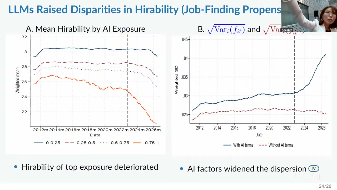
The dispersion of hirability is flat before 2023, then rises steadily and accelerates from 2024. Strip the three ai terms out of the fitted value and recompute the same standard deviation and it is essentially unchanged throughout — flat line, no acceleration, nothing. The ai variables account for 0.5 pp of the level gap and 1.1 pp of the widening after November 2022, 1.6 pp in total. Feed the 1.1 pp through the differenced condition at a 4% unemployment rate and a 0.3 monthly job-finding rate and you get this:

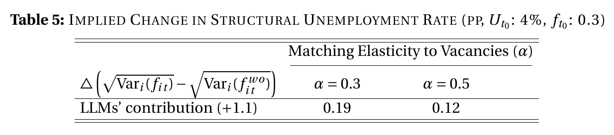
Nineteen basis points at the preferred matching elasticity, twelve at the alternative. Across the robustness designs the range runs from 0.09 pp under three-digit-industry-by-time fixed effects up to roughly half a point under the shift-share adoption-potential instrument, where the estimated widening in dispersion comes out about four times the baseline. The authors’ own sentence is that llms “likely boosted structural unemployment rate by about 0.1–0.2 percentage point.”

The second road, and the band that matters. The other route to the same destination does not use the theory at all. Each group’s separation and job-finding rates go through a Bayesian trend-cycle decomposition — integrated random-walk trends, a Harvey trigonometric cycle at a 36-month period with damping 0.90, the Covid window from March 2020 through December 2021 simply treated as missing — and the trend components go through the two-state steady state to give each group its own natural rate, aggregated with time-varying labour-force shares, draw by draw so that posterior uncertainty propagates. Then you freeze groups at their December 2022 values and see what the aggregate does.

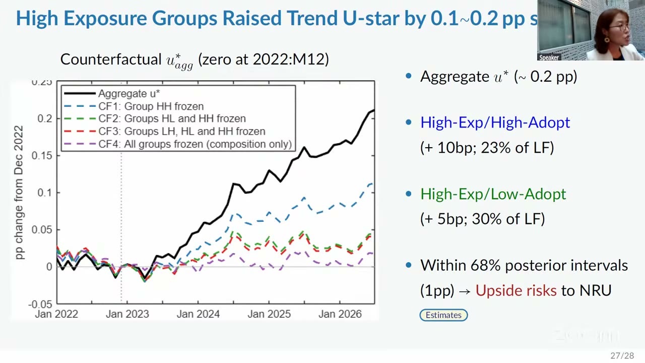
The aggregate trend is up about 0.2 pp since December 2022. Freezing the high-high group removes 0.1 pp of it; additionally freezing high-exposure/low-adoption removes about another five basis points; so high-exposure workers together account for about 0.15 pp. At the group level, high-high’s own natural rate is up about 0.44 pp and high-low’s about 0.23 pp, and the decomposition of that is the same story as everywhere else in the paper — the job-finding trends fall several points while the separation trends barely move.

And then, immediately, the sentence that has to travel with the number or the number should not travel: “Nonetheless, the estimates are subject to considerable uncertainty: the 68% posterior intervals span about 1 percentage point, well exceeding the estimated llm effects. We therefore interpret our results as indicating upside risks to the natural rate of unemployment associated with llms.” Ahn said the same thing out loud with time already up — “these estimates are within the 68 percent of the posterior intervals so not that statistically significant, hence we interpret this result as just suggesting upside risk to the natural rate of unemployment” — and the slide said it too. So the honest summary is genuinely awkward to phrase and that is not the authors’ fault: there is a calibrated 0.1–0.2 pp from the theory, a posterior-mean decomposition of about 0.15 pp from the statistics, the two agree, and the band around the second is wide enough to swallow both. “A Fed paper says ai raised the natural rate by a tenth or two” is a defensible sentence only with the band attached. Without it, it is an overclaim. “They found nothing” is not an improvement.

Two supporting results are worth a line each. The ai wage and hours premium is real and it is fading: exposure and adoption both predicted faster wage growth and more hours before the llms, and the post-2023 interactions run the other way — though the authors point out themselves that the adoption half of the wage reversal loses significance once industry fixed effects go in, and so may be an industry trend rather than adoption per se. And the composition of who is in trouble is not the one the newspapers have: among permanent job losers, the high-high share rose from 23.4% to 32.4% overall, and among college-educated 55- to 64-year-olds it went from 37.0% to 55.4% in three years, which the paper reads as llms possibly affecting labour supply decisions near retirement. The literature’s stock character is a 22-year-old who cannot get an entry-level coding job. He is in there, but he is not the biggest number on the page.

The discussant did not go easy. Gad Levanon of the Burning Glass Institute had both papers in the session, and opened with a disclosure that should be preserved. His organisation is not the Burning Glass that became Lightcast, whose data both papers use; they share a name only because Matt Sigelman runs both. “If anything, there is a mutual feeling of hostility and animosity between the organizations. They indeed sued us to want us to change our name.” He then noted his bias going in and proceeded to give the most useful quarter of an hour of the session.

He conceded the thing that matters first. On whether ai has displaced jobs: “I think the answer is yes. The big question is how much. I think it’s above 100,000 and below 5 million. How did I get to those numbers? I made them up” — but 95% of the room would accept the range, and a hundred thousand is a very different world from five million. And: “no studies found aggregate effect, and some found for young workers in most exposed jobs, but this paper did find aggregate effect.” That is the discussant of record certifying that the paper has done something nobody else has.

Then he took the exposure measure apart. The Eloundou and Felten scores “have very little to do with job displacement. So any paper that uses those measures — it will be a miracle to find a significant impact.” He has worked with them himself; they capture “such a tiny part of how ai is impacting the labor market, so using it as the sole proxy is a non-starter in my opinion.” Adding adoption is “the big idea here” and a step in the right direction, because even where the technology exists, if employers make no effort to adopt it you will see nothing in the labour market — and he believes the interaction does work. But the adoption measure as built “is more of a function of the occupation distribution of each industry,” which would mean it is partly re-measuring which occupations each industry employs rather than how much ai each industry uses. He offered to help build a better one. He asked for a single consolidated table of all specifications against all outcomes, “otherwise it’s hard to tell what’s really happening here.” He endorsed the move to the cps as exactly right, because you see flows and not just stocks and the results look stronger in flows, and told them to do it on the acs and oews too. His closing line was aimed past the authors: “the results are only as good as the exposure and adoption measures behind them. And that’s not just for this paper but for the community at large — you are bound to fail if that’s your exposure measure, that’s how you measure the impact of ai.”

He is right that this is the binding constraint, and it is worth noticing what it implies about the finding. If the exposure measure is as noisy as he says, the attenuation runs against the paper. An uphill climb that ends somewhere is still a climb that ended somewhere.

The best question from the floor went at the interaction from the other side. Exposure is a substitution notion, the questioner said, but a firm posting requirements for an ai solution is buying a complement — so why is high-exposure/high-adoption the worst cell? “It’s even more surprising to see that high-high was the biggest effect. I could have easily seen high-low.” That is the sharp version of the objection. If adoption is complementarity, the exposed workers who should be suffering are the ones whose tasks a model can do and whose employer has no ai in the building to do them with.

Ahn’s answer was to refuse the premise rather than to argue the sign. Adoption, in their view, measures demand for ai-using roles, “but we didn’t make any assumption about whether it’s a complement or a substitute … so it’s an empirical question,” and the empirical answer is that high-high workers’ unemployment rose the most and their job-finding fell the most. On Levanon’s occupation-mix objection — whether aggregating exposure to the industry level would just reproduce the adoption measure — she called it an important question and left it open, which is the correct answer to a question you have not run. Her defence of the interaction was the best sixty seconds of the session, and it was two examples with no algebra in them: managers in construction against managers in computer services, teachers in K-12 schools against teachers in colleges and universities. Same occupation, therefore the same exposure score; different industry, therefore different adoption; different labour market outcomes. Whatever the adoption variable is measuring, it is not constant within an occupation, and that is the margin the literature has not looked at.

Nobody asked about the natural rate. Not the Bayesian decomposition, not the Jackman–Roper extension, not the counterfactuals, not the band. The entire discussion period went on whether the two ai scores mean anything — which is the right question, and also means the one number in the paper with a Federal Reserve Board letterhead on it and a percentage sign after it left the room completely unexamined. It is, of course, the one that is going to get quoted.