The Economics of Density: Evidence From the Berlin Wall

Gabriel M. Ahlfeldt, Stephen J. Redding, Daniel M. Sturm and Nikolaus Wolf, Econometrica, November 2015 (vol. 83, no. 6, pp. 2127–2189). There is no talk or discussant for this paper. Version used: the published article plus the online supplement.

The problem with dense places

The Ahlfeldt–Redding–Sturm–Wolf paper on the Berlin Wall is a way of getting the city to tell you something it normally won’t. Every urban economist knows the problem. Land in the centre of a city is expensive and full of jobs. Either density itself makes the people there more productive and the neighbourhood nicer to live in, or the centre was a good place to begin with (a river crossing, a palace, a railway terminus) and the density just followed the fundamentals. A cross-section can’t tell those stories apart, because in a cross-section the good places and the dense places are the same places. What you would like is to keep the ground under a block exactly as it is and take its neighbours away.

In 1944–45 the Allies did that for you. They drew sector boundaries along 1938 district lines, for military and diplomatic reasons that had nothing to do with land values. The Soviet sector got Mitte, which held the pre-war central business district around Friedrichstrasse and Leipziger Strasse and, in the paper’s words, “by far the largest pre-war concentration of employment” in the city. Economic separation was largely complete by the 1950s and the Wall made it physical in 1961. For a West Berlin block a few hundred metres from Mitte, the surrounding economic mass disappeared while the block itself stayed put. Then in 1989–90 the mass came back. That gives you two shocks, one each way, and the paper uses both.

The authors work only on the West side, where a land market kept operating. East Berlin under central planning is not treated as a market equilibrium. The question becomes how land prices and employment in West Berlin blocks responded to losing, and then regaining, access to a centre across the Wall. Answering it takes a model, and most of the paper is about building one that can be inverted.

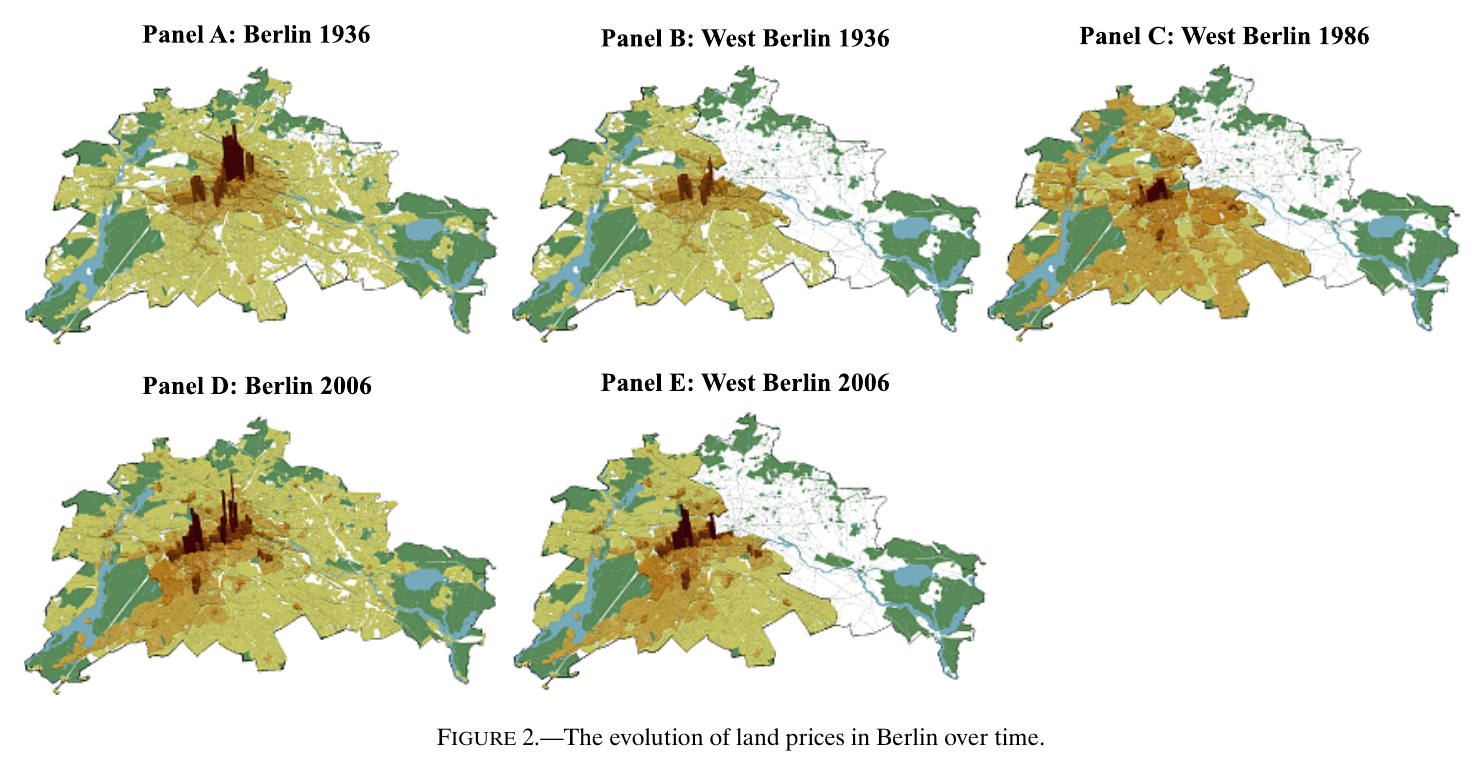
Figure 2 is the whole paper as a land-price surface. In 1936 there is one dominant peak, in Mitte. West Berlin has two smaller high-value areas, one just west of Potsdamer Platz around Anhalter Bahnhof and one on the Kudamm. Under division the Potsdamer Platz area is wiped out and the Kudamm becomes West Berlin’s centre. After reunification Potsdamer Platz comes back and Mitte re-emerges. The point is that the peak near the Wall depended on what was on the other side of the Wall.

The model

The model has no monocentric assumption, and the central business district is an outcome of the equilibrium rather than something imposed. The city is 15,937 blocks (the 2006 geography, fewer than 9,000 of them in West Berlin), each with a land area $K_i$, a floor-space stock, and a travel time $\tau_{ij}$ in minutes to every other block. Workers are freely mobile between Berlin and the rest of Germany, which pins their expected utility at a reservation level $\bar U$. Each worker picks a residence–workplace pair. Utility is Cobb–Douglas over a traded good and residential floor space, times an amenity $B_i$ at the residence, times an idiosyncratic Fréchet draw for that particular pair, divided by an iceberg commuting cost $d_{ij}=e^{\kappa\tau_{ij}}$. The Fréchet draw does the usual job of turning a discrete choice into smooth shares, and the shares give a semi-log gravity equation for commuting. That equation identifies only the product $\nu=\varepsilon\kappa$, where $\varepsilon$ is the Fréchet shape. Firms produce the one traded good with labour and commercial floor space, and zero profit ties a block’s productivity to its wage and floor price. Floor space is built competitively from capital and land and split between commercial and residential use, with a block-specific regulatory wedge. Land rents go to absentee landlords, which keeps the welfare accounting simple at the cost of some realism.

The labour market for blocks clears through commuting:

Here $H_{Mj}$ is employment at workplace $j$, $H_{Ri}$ the number of workers living in $i$, $w_j$ the wage, $E_j$ the Fréchet scale for workplace $j$ and $d_{ij}=e^{\kappa\tau_{ij}}$ the commuting cost; this is equation (7) in the paper, and in estimation form (26) it is written in terms of transformed wages $\omega_j=E_jw_j^{\varepsilon}$.

The agglomeration forces are where the paper makes its choices. There are two of them, each with a size and a reach:

In equations (20) and (21), productivity $A_j$ is a fundamental $a_j$ times a travel-time-discounted sum $\Upsilon_j$ of nearby workplace employment per unit of land, with elasticity $\lambda$ and per-minute decay $\delta$, and amenities $B_i$ are a fundamental $b_i$ times the analogous sum $\Omega_i$ over residence employment, with elasticity $\eta$ and decay $\rho$. These are reduced-form externalities. Nothing in the model says whether $\lambda$ is knowledge spillovers or input sharing, and $\eta$ is a net effect: shops and cafés minus congestion and crime, all at once. The dispersion forces are commuting costs and the inelastic supply of land.

In this model, division means infinite commuting costs, infinite trade costs and infinite spillover decay across the Wall. A West block near Mitte then loses four things: the jobs in the East its residents could commute to, the Eastern residents who commuted in, the production spillovers from Eastern employment, and the residential spillovers from Eastern residents. All four bite hardest close to the Wall near the old centre. So the model predicts that land prices and employment fall there relative to the rest of West Berlin, and that West Berlin as a whole loses people to West Germany. (It did: 2,683,099 in 1933, 2,012,709 in 1987.) Reunification reverses the channels, though not necessarily symmetrically. With agglomeration there can be multiple equilibria, and East Berlin’s own activity had changed in the meantime.

Inverting the city

The structural move is this. Take observed floor prices $\mathbb{Q}$, workplace employment $H_M$, residence employment $H_R$, land areas and travel times, plus parameter values. Proposition 2 says the model then maps uniquely back to the unobserved characteristics of every block, whether or not the forward model has multiple equilibria. The inversion runs in steps. Given $\nu$, the commuting-clearing condition (7) delivers a unique vector of transformed wages $\omega_j$ (a gross-substitutes argument, Lemmas S.6–S.7 in the online supplement), normalised to a geometric mean of one; the wage level is not separately identified from $E_j$. Zero profit plus $\omega$ and floor prices then gives adjusted productivity $\tilde A$. Residential choice plus mobility gives adjusted amenities $\tilde B$, and land-market clearing gives adjusted density of development $\tilde\varphi$. None of this needs a functional form for the spillovers. Only at the last step, given $(\lambda,\delta,\eta,\rho)$, do you strip the spillovers out: $\tilde a=\tilde A\,\Upsilon^{-\lambda}$ and $\tilde b=\tilde B\,\Omega^{-\eta}$. The tildes are an admission rather than a decoration. The adjusted objects absorb the Fréchet scales and the zoning wedge, so those primitives are never separately identified, and the paper says so.

Fundamentals here are structural residuals. Whatever the spillovers can’t explain about a block’s prices and employment is labelled “fundamentals”. That would be circular if nothing disciplined the spillover parameters. The discipline comes from the Wall. In changes, the residuals are

In equations (30) and (31), $\tilde a$ and $\tilde b$ are adjusted production and residential fundamentals, $\mathbb{Q}$ the observed floor price, $\omega$ the transformed wage, $W_{it}$ commuting market access ($\sum_s\omega_{st}e^{-\nu\tau_{ist}}$, equation 29), $1-\alpha$ and $1-\beta$ the commercial and residential floor-space shares, bars geometric means across blocks in year $t$, and $\Delta$ the change across division or reunification. The identifying moments then say that these changes are unrelated to distance from the pre-war cbd:

In equations (32)–(33), $\mathbb{I}_k$ indicates the $k$-th of $K_{\mathbb I}=50$ percentile bins of distance to the pre-war cbd.

Read in English, the moments say: choose the strength and reach of the spillovers so that, after the model’s channels have done their work, nothing systematic about the old-centre gradient is left for “the fundamentals changed” to explain. This is an exclusion restriction on changes in adjusted fundamentals. Any time-invariant part of a block is differenced out, so the paper does not assume fundamentals are constant. It does assume that whatever changed in them between 1936 and 1986 was not arranged by distance to Friedrichstrasse. The military origin of the boundary makes the shock itself plausibly exogenous. It does not by itself deliver that stronger restriction, and keeping those two claims apart matters for the objections below. Two more moments complete the system: the share of commutes under 30 minutes pins $\nu$, and the variance of 1986 West Berlin district wages pins $\varepsilon$. What separates production from residential spillovers is the exclusion structure: workplace density enters only productivity, and residence density enters only amenities.

The reduced form: what the Wall did

Before any of that machinery, the paper runs a plain difference-in-differences. The change in log floor prices (or employment) for West Berlin blocks is regressed on six 500-metre cells of distance to the pre-war cbd, with blocks beyond 3.75 km as the omitted group. The first cell runs to 1.25 km because the nearest West block is about 0.75 km from the cbd. Standard errors are Conley (1999) spatial hac with a 0.5 km cutoff. The cells are small: 23, 37, 50, 84, 146 and 173 blocks. Every coefficient is relative to distant West Berlin, not an absolute loss.

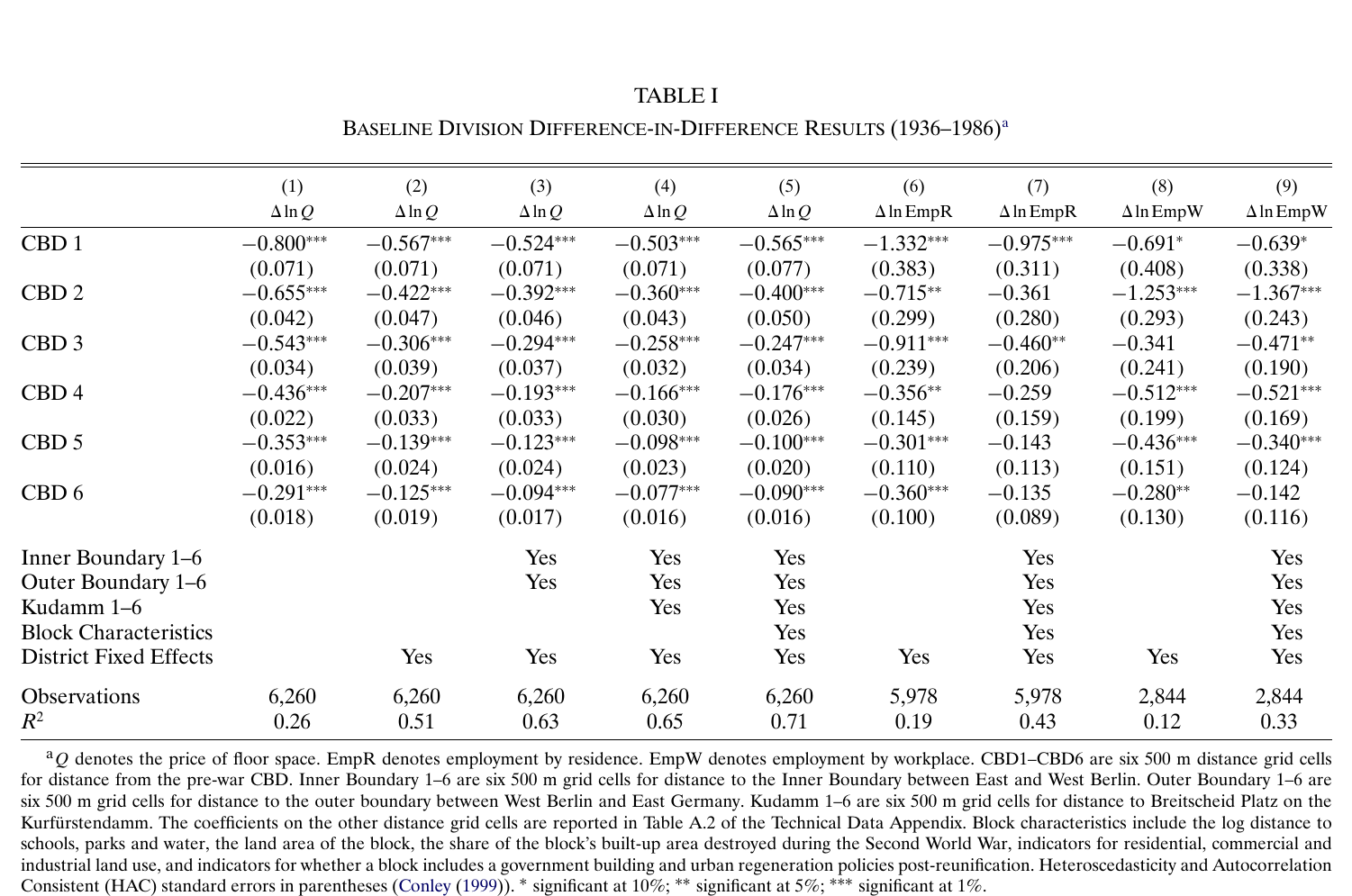
Under division (Table I), floor prices in the nearest cell fall by 0.800 log points (s.e. 0.071), about 55 percent relative to distant blocks, and the effect declines monotonically across the cells: −0.655, −0.543, −0.436, −0.353, −0.291. Adding district fixed effects brings the nearest-cell coefficient to −0.567. Adding cells for distance to the inner and outer boundaries brings it to −0.524, cells for the Kudamm to −0.503, and a full set of block controls to −0.565 (s.e. 0.077). The controls include wwii destruction, government buildings, regeneration areas, land use and distance to schools, parks and water. Residence employment in the nearest cell falls by 1.332 log points, or 0.975 with controls. Workplace employment falls by 0.691 or 0.639, significant only at 10 percent, with larger falls in the second cell. The control columns are the important ones. Distance to the Wall as such has roughly zero effect; distance to the old centre is what matters. A block next to the Wall in the far north of the city did not suffer the way a block next to the Wall by Potsdamer Platz did.

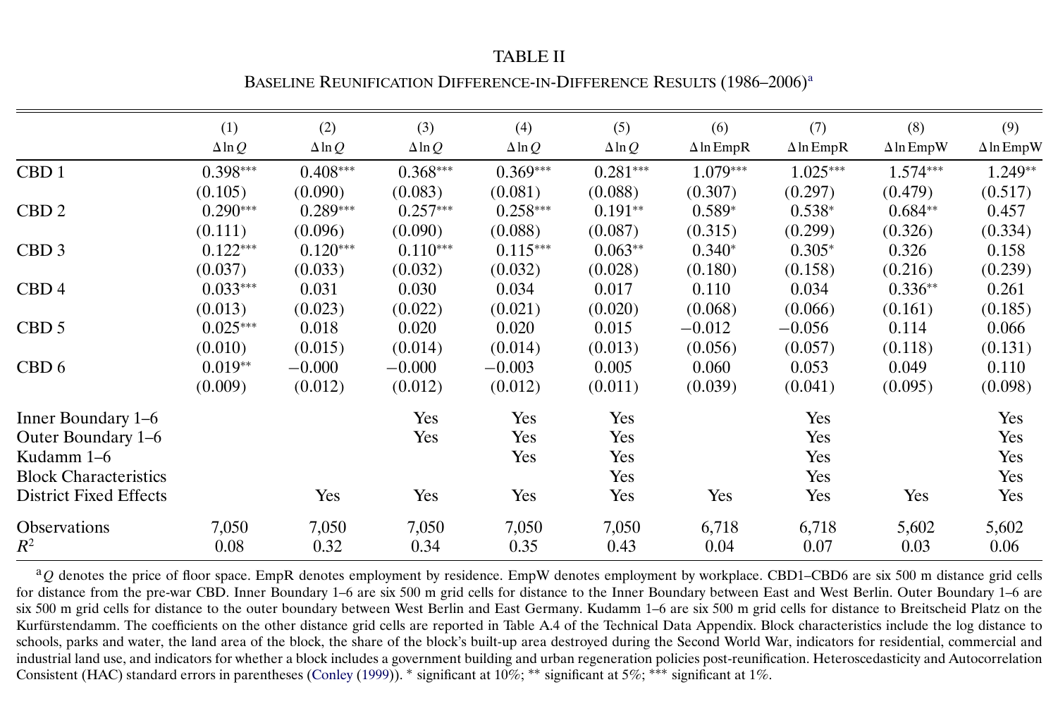
Reunification (Table II) runs the film backwards, but shorter. Floor prices in the nearest cell rise by 0.398 log points (s.e. 0.105), about 49 percent, then 0.290 and 0.122 in the next two cells, and close to zero beyond. With controls the nearest-cell effect ranges from 0.408 down to 0.281. Residence employment rises by 1.079 and workplace employment by 1.574 log points, though the R² values are low. Across blocks, 1986–2006 floor-price growth regressed on 1936–86 growth gives −0.262: the places that lost the most gained back the most.

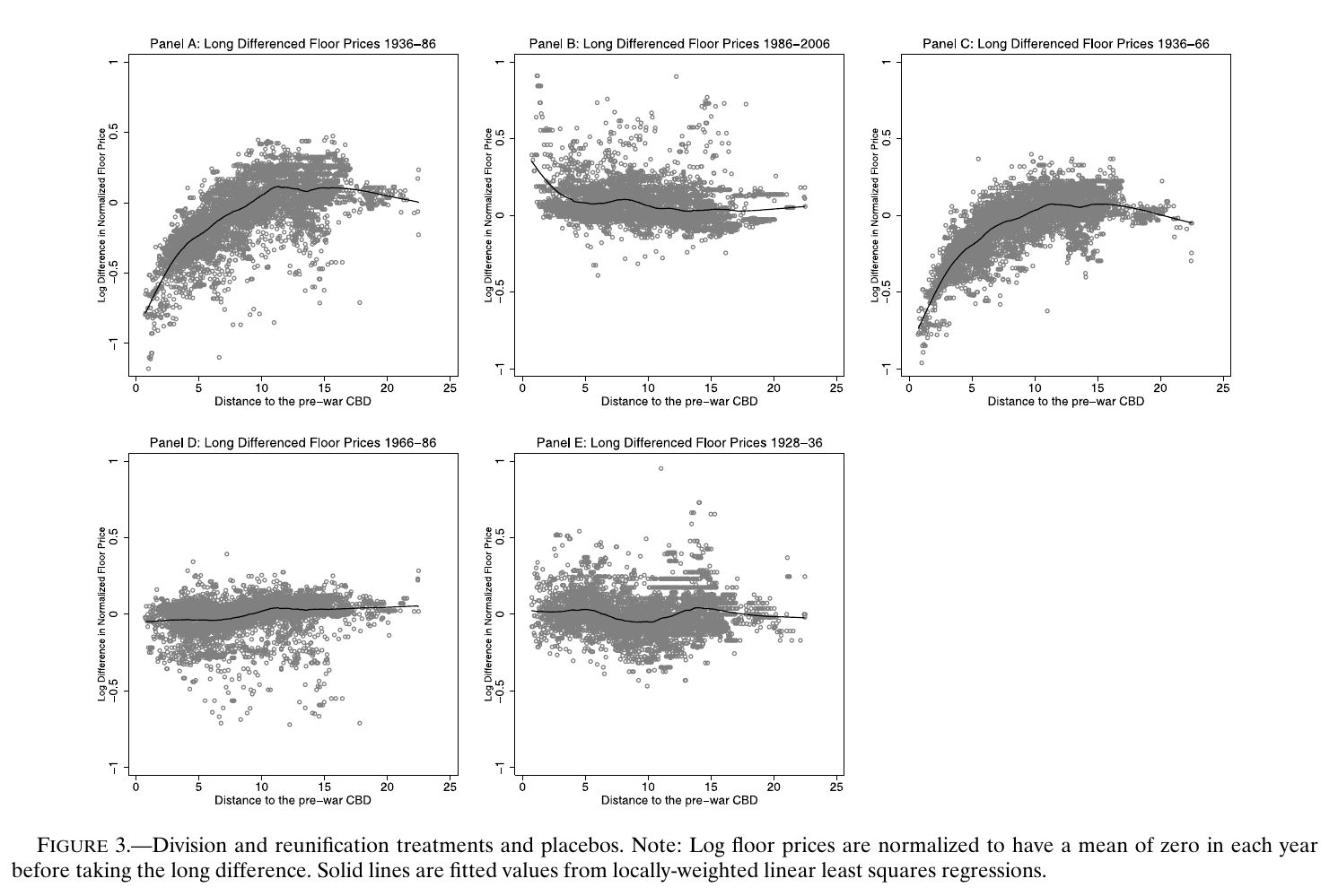
Figure 3 adds the timing. Most of the division effect was already in place by 1966. From 1966 to 1986 the gradient is flat, so there is no pre-trend before reunification, and from 1928 to 1936 it is flat too, so there is no pre-war pre-trend. That rules out the particular pre-trends you would worry about. It is not a proof of parallel trends, since nobody observes what Potsdamer Platz would have done after 1945 without the Wall.

Commuting parameters

The commuting side is estimated from a 2008 survey of trips between Berlin’s twelve districts, which gives 144 origin–destination cells.

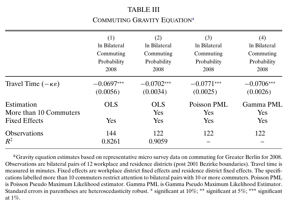
With residence and workplace fixed effects, the travel-time coefficient is −0.0697 by ols (R² 0.83), −0.0702 on the 122 cells with at least ten commuters, −0.0771 by Poisson pml and −0.0706 by Gamma pml. So $\nu\approx0.07$, a semi-elasticity per minute (Table V calls it an elasticity, which it isn’t): each extra minute cuts commuting by about 7 percent. The data are district-level and the model is block-level, so there is an aggregation problem; the authors report that data simulated with $\nu=0.07$ re-estimate at 0.0726, a check they document in their separate Technical Data Appendix, which we did not see.

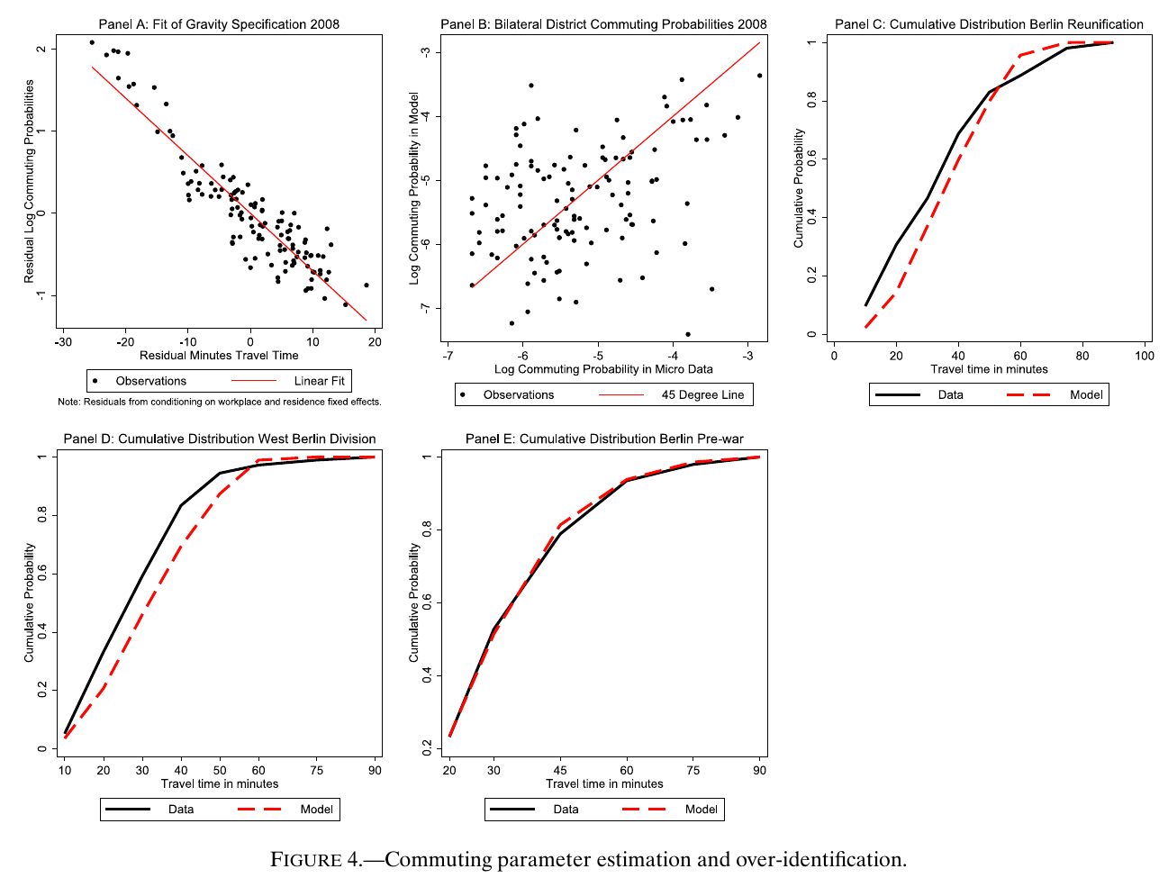
Figure 4 shows that the residualised log commuting shares are close to linear in residual travel time. With the single 2008 $\nu$, the model reproduces the binned distribution of commuting times not only in 2008 but in West Berlin in 1986 and in pre-war Berlin. The early bins fit less exactly in the later years than in 1936. These historical distributions are over-identification checks on the gravity estimate. The under-30-minute share later becomes a gmm moment, so in that role it is not an independent test.

The Fréchet shape comes from wages. In the model the variance of log adjusted wages is $(1/\varepsilon)^2$ times the variance of log transformed wages, and matching the 1986 variance of blue-collar manufacturing wages across West Berlin districts (the largest gap between districts is 26 percent) gives $\varepsilon=6.83$. That sits comfortably inside the Eaton–Kortum (2002) range of 3.60 to 12.86, and it implies $\kappa=\nu/\varepsilon\approx0.01$. The three expenditure and cost shares are calibrated from the literature rather than estimated: a housing share $1-\beta=0.25$, a commercial floor-space share $1-\alpha=0.20$ and a land share in construction $1-\mu=0.25$.

The model without agglomeration fails, informatively

Now run the inversion with the spillovers switched off and see what the “fundamentals” do.

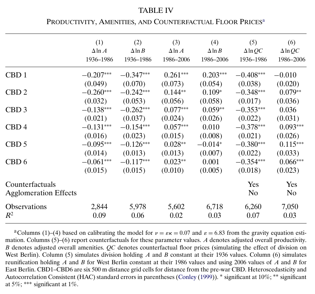
Recovered adjusted productivity in the nearest cell falls by 0.207 log points under division and adjusted amenities by 0.347. Under reunification they rise by 0.261 and 0.203. Fundamentals that are actually fundamental should not care how far a block is from a cbd on the other side of a wall. These ones care a lot, and in both directions. That is the model telling you it is missing something.

The counterfactual in the same table makes the point sharper. Hold $\tilde A$, $\tilde B$ and $\tilde\varphi$ fixed at their 1936 values, impose division and let only commuting access respond. (Without agglomeration the equilibrium is unique, by Proposition 1.) The nearest cell then loses 0.408 log points, about half of the observed −0.800. The loss is also nearly flat across the cells: −0.408, −0.348, −0.353, −0.378, −0.380, −0.354. Losing commuters and commuting destinations makes all of West Berlin poorer by roughly the same amount, because at those distances everyone in West Berlin is a few minutes’ tram ride from everyone else. The reunification counterfactual gives −0.010, statistically nothing, against the observed +0.398. Commuting access explains about half of the level of the division effect, none of its gradient and none of the reunification jump. That failure is conditional on the rest of the model, but it is the failure the paper needs.

Estimating the spillovers

The gmm estimation is two-step efficient gmm: identity weights first, then a Conley-hac weighting matrix. It is run separately for division and reunification and then pooled, with the commuting and wage moments from the division era serving both experiments. There is deliberately no moment on development density, since building density could itself respond to the model’s own mechanisms.

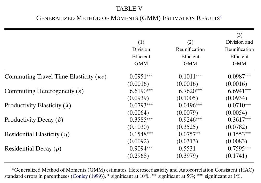
In the preferred pooled column, $\nu=0.0987$, $\varepsilon=6.69$, $\lambda=0.071$ (s.e. 0.005), $\delta=0.36$, $\eta=0.155$ (s.e. 0.008) and $\rho=0.76$. Division alone gives $\lambda=0.079$, $\delta=0.36$, $\eta=0.155$ and $\rho=0.91$. Reunification alone gives smaller elasticities ($\lambda=0.050$, $\eta=0.076$) and noisier estimates: its residential decay $\rho$ is insignificant, and its production decay is faster, at 0.92, not slower. The authors pool on the argument that spillover parameters should be deep, while conceding that the reunification shock is smaller and that technology, industry mix and amenities may have changed. The two sets of estimates are similar in the sense that the elasticities have the same order of magnitude. They are not the same, and the pooled $\delta$ sitting almost exactly at the division value tells you which experiment is doing most of the work. The structural $\nu$ of about 0.10 against the gravity 0.07 is also called “similar” in the text, which is generous. A further wrinkle: the text gives $\kappa$ as “0.01” twice, which is the gravity-route number (and a rounding of the gmm one), while the Table VI note gives the pooled implied value of 0.0148.

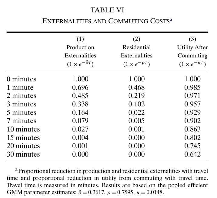
The decay table is where the numbers become physical. A source block’s contribution to production spillovers is weighted 0.696 at one minute’s travel, 0.164 at five minutes, 0.027 at ten and essentially zero at fifteen, which is a half-life of a little under two minutes. Residential spillovers fall faster: 0.468 at one minute, 0.022 at five and 0.001 at ten, a half-life under one minute. Commuting, by contrast, is cheap. Utility after a ten-minute commute is still 0.863 of utility with no commute, and after thirty minutes 0.642. Ten minutes is about 0.83 km on foot or about 4 km by U-Bahn or S-Bahn. The externalities are neighbourhood-sized, while the labour market is city-sized.

The one surprising thing

Here is the result that makes the paper. You might have expected the Wall to hurt West Berlin’s centre mainly through the labour market: half the jobs your residents could reach are gone, so your land is worth less. That channel is real, but Table IV shows it is flat across West Berlin. The steep gradient in the data, the fact that the block 1 km from Mitte lost far more than the block 3 km away, is almost entirely the work of spillovers that reach only a few minutes. Put $\lambda=0.071$ and $\eta=0.155$, with their two-minute and one-minute half-lives, back into the model, hold fundamentals fixed, and simulate.

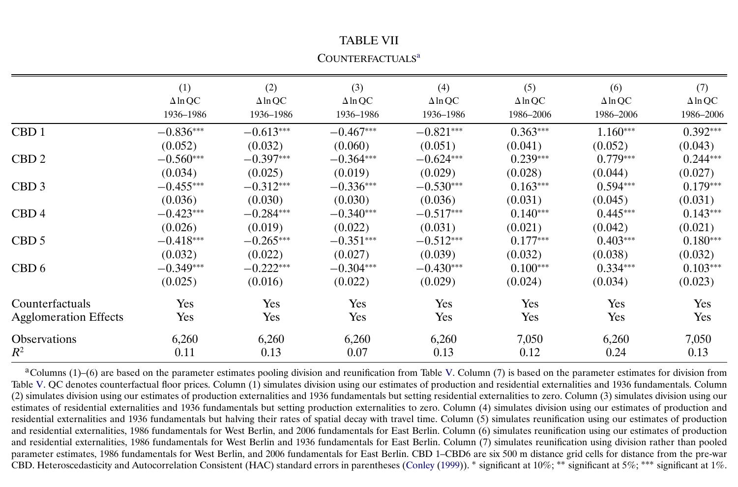
Division with 1936 fundamentals and the pooled parameters gives −0.836 in the nearest cell against −0.800 observed, and the cells after it fall away (−0.560, −0.455, −0.423, −0.418, −0.349 against −0.655, −0.543, −0.436, −0.353, −0.291), slightly over-predicting further out. Reunification with 2006 East Berlin fundamentals gives 0.363 against 0.398. Setting $\eta=0$ shrinks the nearest-cell division effect to −0.613, and setting $\lambda=0$ shrinks it to −0.467. These are not additive shares, but both channels matter, and residential spillovers, which are about as large as production ones and decay faster, carry a big share of the effect. Halving both decay rates barely moves the nearest cell (−0.821) but enlarges effects further out. Equilibrium selection is handled by starting from the observed pre-shock equilibrium and iterating with damping to the “closest” counterfactual equilibrium, and the authors frame these exercises as checks of fit, not unique predictions.

Two qualifications follow from the paper’s own construction. The R² of about 0.11–0.12 under Table VII is the six distance bins explaining simulated block-level changes. It does not measure how well simulated changes track observed changes block by block, and no such comparison is reported. The fit is a coefficient-to-coefficient match on a six-cell distance profile. The second qualification concerns column 6, the most striking number in the table. Swap the 2006 East Berlin fundamentals for the 1936 ones, let Eastern employment and residence adjust, and match the 2006 Berlin population. The nearest-cell reunification coefficient becomes 1.160 log points, about three times the observed 0.398. The authors read this as what a recovery of East Berlin to its pre-war relative development would do. It is a fundamentals swap, not a forecast. Twenty years after reunification, the recovery it describes had not happened.

What the online supplement does

The online supplement is long (75 pages) and does most of the theory. It derives the model, including the isomorphisms that let you read commuting disutility as lost effective labour and Fréchet utility draws as efficiency draws. It proves existence and uniqueness with exogenous fundamentals and the unique-inversion results, and it writes out the counterfactual algorithms. Three parts deserve attention.

The first is data construction, which is where an exercise like this succeeds or fails. Floor prices for 1986 and 2006 come from the Berlin valuation board’s assessed land values for undeveloped land, digitised block by block. For 1936 they come from Kalweit’s street-level land values, matched to blocks in gis. Land values become floor prices through the Cobb–Douglas construction technology, $\mathbb{Q}=\chi R^{1-\mu}$. The supplement validates the modern assessments against 51,275 transactions from 2000 to 2012, using a Case–Shiller-type specification with block fixed effects for 8,907 blocks (R² 0.769). Transaction prices per unit of lot area line up against assessed values with a slope of about one, as does floor-to-land ratio, which supports both the assessments and the construction function. That validation covers only the modern data; nothing comparable exists for 1936. The 1933 workplace employment is constructed. District private-sector totals from the 1933 census are allocated across blocks by counts of firms in the 1931 commercial register (42,818 of 47,098 firms geocoded), so firm size within a district is inferred rather than observed. The district-level fit of log employment on log firms is R² 0.77, and a block-level check with 1987 data gives 0.57. Public employment is placed in buildings by occupation using a 1945 Allied map, so teachers go to schools. The 1933 residents come from census population by street, spread equally over the contiguous blocks.

Travel times are computed as shortest paths over all of roughly 254 million block pairs, separately by year. Public-transport speeds come from a 1928 source and are held constant: 5 km/h walking, 25 for U- and S-Bahn, 14.5 for tram and 14.3 for bus, with a three-minute transfer penalty. Car times come from street speeds and correlate 0.94 with Google’s estimates, though Google’s median is 7.9 minutes longer. For 1986 and 2006 the two modes are mixed using a district-level car share fitted to modal-split data from around 2010, with the same weights reused for 1986; cars are about a third of trips. 1936 uses public transport only. The commuting surveys are a 2008 micro survey, a 1982 survey of 291 West Berlin households, and a late-1930s study of 24,336 workers at eight workplaces. (The published version counts 7,948 commuters in the 2008 survey and the online supplement 7,984; one of them has transposed digits.)

The second is the structural estimation itself. Own blocks are excluded from $\Upsilon$ and $\Omega$ in estimation, “to rule out a mechanical correlation”, even though the sums as written in (20)–(21) include them. Computation is a nested fixed point. An inner loop updates transformed wages by the ratio of observed to predicted employment, damped half and half with the old value, and an outer pattern search runs over the parameters. Each evaluation of the moments takes about 30 seconds over the 254 million commuting probabilities, and the full run takes under a day on a cluster. The supplement’s evidence on identification is a set of grid searches. One-dimensional grids for $\nu$ and $\varepsilon$ each show a single minimum, and 20-by-20 grids over $(\lambda,\delta)$ and $(\eta,\rho)$ each show a single bowl.

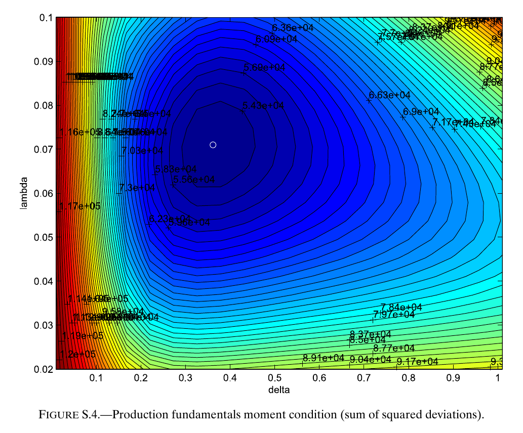
Companion figures show the mean change in recovered fundamentals by distance cell. It is flat at the estimates and sloped when the spillovers are stronger or weaker than estimated, which is the cleanest picture of what the moments are doing. These are conditional grids under the maintained functional forms, not a global identification proof. The Monte Carlo evidence is reported to be in the Technical Data Appendix, which we did not see. There is also a small glitch: the text gives the $\delta$ grid as running “from 0.01 to 0.101”, while the figure’s axis runs to about one and the estimate is 0.36, so presumably 0.01 to 1.01 was meant. Elsewhere, 3,984 blocks are said to give “1.59 million” matrix elements when the square is about 15.9 million.

The third part is robustness and an extra counterfactual. Most of the empirical robustness lives in the Technical Data Appendix, not in the online supplement. According to the paper, that appendix contains standard errors clustered on statistical areas, alternative controls, subperiod regressions, variation in U- and S-Bahn access, and two over-identification checks. One is a slope of 0.959 between the model-implied and observed floor-to-land ratio in 2006. The other shows that recovered amenities are higher near green space, water and listed buildings and lower near noise and wwii destruction. We report these as the paper describes them; we have not checked them. What the online supplement does contain is a transport-technology counterfactual.

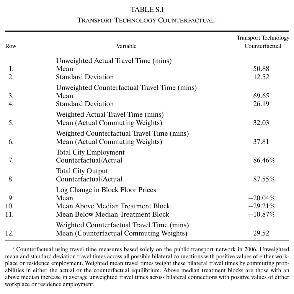
Take 2006 Berlin and remove cars, so everyone travels on 2006 public transport, while holding fundamentals and floor space fixed and letting people leave for the rest of Germany. The unweighted mean block-to-block travel time rises from 50.88 to 69.65 minutes, and from 32.03 to 37.81 minutes at the actual commuting weights. City employment falls to 86.46 percent of actual and output to 87.55 percent. The mean log floor-price change is −0.20: −0.29 for blocks whose travel times rise by more than the median and −0.11 for the rest. Blocks also become less specialised as places to work or to live. The neat part is that the average commute at the counterfactual weights is 29.52 minutes, shorter than the actual 32.03. Worse transport produces shorter commutes, because people re-sort into nearby jobs and some leave the city. A shorter average commute is not evidence of higher welfare. Unlike Table VII, this exercise is a genuine prediction, so it inherits the equilibrium-selection caveat in full.

Objections and limits

A note on objections, ours rather than a discussant’s: the most important weakness is the exclusion restriction. The moments require the entire old-centre gradient in changes of fundamentals to be zero. The block controls (war destruction, government buildings, regeneration areas) enter only the reduced form, not the gmm. So any real change in fundamentals arranged by distance to Mitte loads straight onto $\lambda$ and $\eta$. Candidates include the death strip being nastier near the centre, heavier bombing in the centre, the government’s return after 1991, or the Potsdamer Platz megaproject. The flat placebo windows and the near-zero Wall-proximity effect argue against this, but they cannot observe the post-war counterfactual. Second, measurement. The 1936 economy is partly constructed, and those constructed densities feed into $\Upsilon$, $\Omega$ and the wages from commuting clearing, so measurement error enters every spillover parameter. In this nonlinear system neither the sign nor the size of the resulting bias is established, and the paper does not analyse it. Excluding own blocks deals with mechanical correlation, not with error. Third, the commuting side is thin: one 2008 survey at twelve districts, imposed on 1936 and 1986, and a Fréchet shape resting on one variance of manufacturing wages across about a dozen districts. The travel times are engineered too, with 1928 speeds held fixed for seventy years and car shares from around 2010 reused for 1986. Spillovers decay in minutes, so $\delta$ and $\rho$ inherit any error in those minutes.

Beyond those, the functional form does a lot of the separating. Workplace density affects only productivity and residence density only amenities, there are no cross-spillovers, decay is exponential, and everything is Cobb–Douglas with a single traded good. The calibrated shares are held fixed for seventy years with no sensitivity analysis in the online supplement. The two experiments give visibly different spillover parameters before they are pooled. The baseline fits exactly by construction of the inversion, so the gradient comparison in Table VII is the real test, and it shares its distance structure with the estimating moments. And the estimates are local in a specific sense. $\lambda$ is the response of productivity to surrounding workplace density holding the travel-time geography fixed. It is not the elasticity of productivity with respect to city size, a point the paper makes itself: double a city and it spreads out. Later work has pushed on the granularity of commuting flows, uniqueness and skill sorting. That is our framing, not the paper’s.

None of this undoes the central result, which is unusually well engineered for its field. A city split for reasons unrelated to its economy, two shocks in opposite directions, and a structural model that can be inverted without solving for equilibrium together give a credible answer to a question that cross-sections cannot touch. The answer is that density pays, but only within a short walk. A Berlin block cared a great deal about the office buildings three minutes away and hardly at all about those fifteen minutes away. For the West Berlin blocks nearest the old centre, the Wall cut them off from exactly the neighbours that were within that range.

References