A Model of Growth Through Creative Destruction

Philippe Aghion and Peter Howitt, Econometrica 60 (2), March 1992, pp. 323–351. Digested from the published version; no recorded talk or discussant (the 2025 Nobel lectures cover the wider research programme, not this paper, and were not used).

Aghion and Howitt’s paper is the one that put Schumpeter’s creative destruction into an endogenous growth model, and the thing to notice first is what that does to the price of an idea. In Romer (1990) a new design is a new variety, it sits beside the old ones, and its owner collects a markup forever. Here a new design is a better version of the one thing the economy uses, so it makes the old one worthless, and its owner collects a markup only until somebody makes it worthless in turn. A patent stops being a perpetuity and becomes a perpetuity with a default intensity, and the default intensity is set by how much research everyone else is going to do. That one change is the whole paper. It makes today’s research depend on expected research tomorrow, it turns equilibrium into a forward-looking difference equation of the kind monetary theorists know from overlapping-generations models, and it lets laissez-faire growth come out too fast as well as too slow.

The authors open by quoting Schumpeter on capitalism “incessantly destroying the old one, incessantly creating a new one”, and then do something unusually literal with it. Each innovation is big enough to move the whole economy, the time between innovations is random, and the length of a “period” is simply the life of the current technology. For a reading list about growth and asset pricing, this is the bridge paper: it gives you an economy whose output is a random walk with drift, whose firms are priced by a discount rate with an obsolescence hazard in it, and whose agents are risk neutral, so nothing in it earns a risk premium. That last part is the gap the later papers in the collection were written to fill.

The model: a patent is a bond the next researcher defaults on

Households are risk neutral with a constant rate of time preference $r$, which with linear utility is also the interest rate. There are three kinds of labour: unskilled labour $M$, which only works in the final-good sector and is folded into the production function; specialised labour $R$, which only does research; and skilled labour $N$, which can either do research or make the intermediate good. Final output is $y = A F(x)$ with $F$ concave, and the intermediate good is made one for one from skilled labour, $x = L$. So the only real allocation decision in the economy is how to split $N$ between making the intermediate, $x_t$, and trying to replace it, $n_t$, with $N = n_t + x_t$.

Research is a Poisson lottery. Innovations arrive economy-wide at rate $\lambda\varphi(n)$, with $\varphi$ concave and $\varphi(0) = 0$, so no skilled research means no growth; the “linear” case $\varphi(n) = n$ does a lot of the paper’s concrete work. Research has no memory, so only the current flow matters. Each innovation is a new intermediate good that raises productivity by a factor $\gamma > 1$, so after $t$ innovations $A_t = A_0\gamma^t$. The inventor gets an infinitely-lived patent, which sounds generous until you notice that the patent covers a good nobody will want once the next one arrives. Until Section 5 innovations are “drastic”: the new monopolist charges its unconstrained price without worrying about the previous vintage.

Within an interval everything is constant. The monopolist faces inverse demand $p_t = A_t F'(x_t)$, sets marginal revenue equal to the productivity-adjusted wage $\omega_t = w_t/A_t$, and earns $\pi_t = A_t\tilde\pi(\omega_t)$, where $\tilde\pi$ is decreasing in the wage. In the Cobb–Douglas case $F = x^\alpha$, the price is $w_t/\alpha$, so $1-\alpha$ is the Lerner index and a measure of market power. Outside research firms hire skilled labour until its wage equals $\lambda\varphi'(n_t)$ times the value of winning, which brings us to the one equation every later asset-pricing paper in this line rewrites:

This is eq. 2.12 in the paper: $V_{t+1}$ is the value of the $(t+1)$-th innovation, $\pi_{t+1}$ its flow monopoly profit, $r$ the interest rate, and $\lambda\varphi(n_{t+1})$ the Poisson arrival rate of the next innovation, which is the rate of creative destruction.

Read it as a credit-risky consol. A constant coupon $\pi_{t+1}$, discounted at the riskless rate plus a hazard of total loss, and the hazard is not a property of the borrower but of the economy: it is how much research will be done next interval. The authors’ “creative destruction” is, quite literally, the second term in that denominator. (Because agents are risk neutral, the spread over $r$ is pure expected loss; there is no risk premium hiding in it. The paper says as much in a different way, noting that a frictionless credit market and paying researchers in shares of the next intermediate firm are equivalent here, because with linear utility no one wants to share risk.)

Two side effects drop out immediately. The incumbent does no research, because its gain from the next innovation is $V_{t+1} - V_t$, less than an outsider’s $V_{t+1}$: Arrow’s (1962) replacement effect, in a model where the incumbent’s own patent is the thing being destroyed. And each innovation raises productivity forever and is the platform for every later one, while its owner collects for one interval: the intertemporal spillover, Romer’s externality, with an expiry date attached.

The difference equation

Put the labour market, the monopolist’s pricing and the research condition together and you get the paper’s central object:

This is eq. 3.1 in the paper: the left side is the marginal cost of research $c(n_t)$, the productivity-adjusted wage $\tilde\omega$ at manufacturing employment $N - n_t$ divided by the marginal arrival rate $\lambda\varphi'(n_t)$, and the right side is the marginal benefit $b(n_{t+1})$, $\gamma$ times next interval’s productivity-adjusted profit discounted at $r$ plus next interval’s rate of creative destruction.

The cost depends on today’s research and rises with it. The benefit depends only on tomorrow’s research and falls with it, for two reasons, and the paper is careful to keep them separate. The first is the denominator: more research next interval means a shorter expected monopoly. The second is the wage: more research next interval means less skilled labour making the intermediate, a higher skilled wage, and a smaller flow of rents $\tilde\pi$ for whoever holds the patent. So eq. 3.1 defines a decreasing map $n_t = \psi(n_{t+1})$ (eq. 3.2): expect a research boom tomorrow, and you do less research today. That is the paper’s surprising thing, and it is worth saying slowly. The reward to an innovation is a rent stream that the next wave of innovators will destroy, so the expectation of vigorous innovation is itself a deterrent to innovating. In the patent-race literature the prize was a number; here it is a price that depends on everyone’s beliefs about the next race.

A stationary equilibrium is a fixed point $\hat n = \psi(\hat n)$:

This is eq. 3.3 in the paper: $\hat n$ is stationary research employment, at which the marginal cost and marginal benefit of research coincide when both today and tomorrow have the same research.

Because cost rises and benefit falls, the stationary equilibrium exists and is unique. It has positive research if $c(0) < b(0)$, and zero research, and no growth ever, if $c(0) \geq b(0)$. (The text states the zero case once as “$c(0) \leq b(0)$” on p. 332, a typo it corrects on the next page.) In the linear Cobb–Douglas case the condition collapses to $1 = \lambda\gamma\left(\frac{1-\alpha}{\alpha}\right)(N-\hat n)/(r+\lambda\hat n)$, eq. 3.4, which you can solve in your head.

Cycles and the no-growth trap

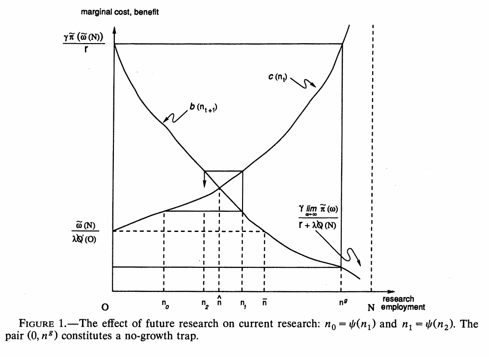
A decreasing map is exactly the thing that can produce oscillation, and Figure 1 draws it. Start at some $n_0$, read off the benefit level it must match, find the $n_1$ that delivers that benefit, and repeat: the perfect-foresight path spirals around $\hat n$. The paper notes that this is the same structure as the two-period overlapping-generations money model of Azariadis (1981) and Grandmont (1985), which is a nice irony, since the model has no money and no generations.

That opens the door to two-cycles, pairs with $n^0 = \psi(n^1)$ and $n^1 = \psi(n^0)$. If both are positive you get a “real” two-cycle, in which expected high research in odd intervals discourages research in even ones, and expected low research in even intervals encourages it in odd ones. If one of them is zero you get what the authors call a no-growth trap, the outer rectangle in Figure 1 running from $0$ to $n^g$. Here the expectation that the next innovation will be followed by a burst of research is enough to stop anyone making that innovation. And since research is zero, the innovation never comes, the “period” never ends, and the promised burst never has to be delivered. Growth stops in finite time, sustained entirely by a belief about an interval that never starts.

The conditions matter, and the paper states them as sufficient conditions, not as a description of where economies sit. A no-growth trap exists if $\tilde\pi(\omega) \to 0$ as $\omega \to \infty$ and $r$ is small enough. A real two-cycle exists if a no-growth trap exists and $c'(\hat n) + b'(\hat n) > 0$. In the linear Cobb–Douglas case that means a trap when $r$ is small and a real two-cycle when $\alpha$ and $r$ are both small enough. The authors also distinguish these cycles from Shleifer’s (1986) implementation cycles: there is no contemporaneous strategic complementarity here, only the dependence of today on tomorrow. Having shown that cycles can exist, the paper then studies stationary equilibria for the rest of its length.

GNP as a random walk with drift

On the stationary path, output in interval $t$ is $y_t = A_t F(N - \hat n)$, so each innovation multiplies output by $\gamma$. Log output is a step function: steps of size $\ln\gamma$ at exponential waiting times with rate $\lambda\varphi(\hat n)$. Sample it at unit intervals and the number of steps in each interval is Poisson, so log gnp is a random walk with drift (eqs. 3.8–3.10), and the paper’s growth moments are just the moments of a compound Poisson process:

This is eq. 3.11 in the paper: $\lambda\varphi(\hat n)$ is the stationary Poisson arrival rate of innovations and $\ln\gamma$ the log step size of each innovation.

For anyone coming from asset pricing, this is the useful part and also the limiting part. The model delivers a unit root in output endogenously, with shocks that are permanent because each innovation is. But the mean and the variance of growth are driven by the same Poisson process, so their ratio is pinned at $\ln\gamma$, and every comparative static that raises average growth raises its variance too. Proposition 1 says stationary research rises with a lower $r$, a larger step $\gamma$, a larger skilled labour force $N$ and a more productive research technology $\lambda$. The last one is not automatic, because a higher $\lambda$ also raises the expected rate of creative destruction next interval; the authors’ resolution is that the cost effect, as they put it, “dominates”. In the Cobb–Douglas case more market power (a smaller $\alpha$) also raises research, and some minimum degree of market power is needed for any growth at all. (The paper prints the threshold as $\alpha < \lambda\gamma N/(\lambda\gamma N + 1)$; its own eq. 3.5 rearranges to $\lambda\gamma N/(\lambda\gamma N + r)$, so the printed version is right only at $r = 1$. The qualitative point does not depend on it.) All of these move agr and vgr the same way. The positive dependence on $N$ is the scale effect, which will matter later.

The paper then lets $\lambda$ be random, drawn afresh at each innovation, with a high state meant as a “fundamental breakthrough” and a low state as an exhausted line of research. Making research more productive in one state can deter research in the others, because it raises the creative-destruction hazard faced by their innovations. The text keeps this hedged (“might raise”, “would tend to reduce”), and the hard result is a single limiting example in Appendix 1. With two states, every transition probability equal to one half, linear $\varphi$, $\alpha = \gamma^{-1} = 1/2$ and $r = N = \lambda_1 = 1$, setting $\lambda_2 = 1$ gives average research $1/3$ and an average growth rate of $(1/3)\ln 2$. As $\lambda_2 \to \infty$, research in the low state goes to zero, the economy spends almost all its time in the low state, and average growth goes to zero. An unambiguous improvement in research technology can, in the limit, abolish growth, because it makes every other innovation a bond with a terrible default rate.

Too much growth, or too little

The planner maximises expected discounted consumption, and since each innovation scales output by $\gamma$, the optimum is a constant research level $n$. Integrating over the Poisson process gives welfare $U = A_0F(N-n)/\big(r - \lambda\varphi(n)(\gamma-1)\big)$, eq. 4.3, which is finite only as long as that denominator stays positive. That is a Gordon growth formula: a consumption stream that rises by the proportion $\gamma - 1$ at rate $\lambda\varphi(n)$ has expected growth $\lambda\varphi(n)(\gamma-1)$, and a risk-neutral agent capitalises it at $r$ minus that. Set the private and social formulas side by side and the difference is stark: the private discount rate on an innovation is $r + \lambda\varphi(n)$, above $r$, and the social one is $r - \lambda\varphi(n)(\gamma-1)$, below it. The planner’s first-order condition is

This is eq. 4.4 in the paper: $n^*$ is optimal research, $F'(N-n^*)$ the social marginal cost of a research worker, $(\gamma-1)$ the net productivity gain of an innovation, $F(N-n^*)$ total output, and $r - \lambda\varphi(n^*)(\gamma-1)$ the social discount rate.

Compare it term by term with eq. 3.3 and you get four wedges, two in each direction. The discount rate is the intertemporal spillover: the planner counts the benefits of an innovation forever, the private firm only until it is replaced, which makes laissez-faire research too low. Output against profit is appropriability: the innovator gets $\tilde\pi$, not $F$, which also makes research too low. Those are the two Romer forces. The new ones push the other way. The planner uses $\gamma - 1$ where the firm uses $\gamma$, because the firm does not care that it is wiping out the previous monopolist’s rents; that is business stealing, and it makes research too high. And the planner values a research worker at her marginal product $F'$, while the firm pays the wage $\tilde\omega$, which is lower because the alternative employer is a monopolist; that is the monopoly distortion, and it also makes research too high.

So laissez-faire growth may be above or below the optimum, and the paper shows that both happen. In the linear Cobb–Douglas case, research is too low when $\gamma$ is large. It is too high when market power is large ($\alpha$ near zero) and $\gamma$ not too large; the paper’s example ($\alpha = 1/2$, $\gamma = \sqrt2$, $r/\lambda N = 2(\sqrt2 - 1)$) has an optimal research level of zero alongside positive equilibrium research. That is the paper’s headline normative point, and it reverses a presumption that Romer-style models had built up: if growth comes from destroying incumbents, private firms may overdo it, because the destruction is a private gain and a social wash.

The later sections test this against relaxations, and it mostly survives. With nondrastic innovations (in Cobb–Douglas, $\gamma < \alpha^{-\alpha}$) the new monopolist limit-prices against the old one, the markup becomes $\gamma^{1/\alpha}$ instead of $1/\alpha$, the comparative statics carry over, and welfare is still ambiguous. When firms choose how big an innovation to aim for, trading size against arrival, private firms maximise arrival times gross size $\gamma$ while the planner maximises arrival times net size $\gamma - 1$, so innovations come out too small; that is business stealing again, wearing a different hat. Its effect on average growth is ambiguous, since smaller steps arrive faster. If the incumbent behaves strategically and hires extra skilled labour to crowd out research and delay its own replacement (in the linear case its wage does not move at all; with concave research the extra hiring also bids up the wage it pays), then in the linear case this monopsony distortion exactly cancels business stealing and linear Cobb–Douglas growth is unambiguously too low. The authors then set it aside as an artefact of having one intermediate firm in the whole economy. With $m$ intermediate sectors innovated in rotation, average growth keeps the form $\lambda\hat n\ln\gamma$ in the linear case, but its variance becomes $\lambda\hat n(\ln\gamma)^2/m$, the law of large numbers doing to aggregate growth what it does to a diversified portfolio. That comparison holds at a given level of research: $\hat n$ itself is solved from a condition that contains $m$, so across equilibria both moments can move.

What is not here

Notice what the model never needs: a price of risk. Households are risk neutral, so the patent’s discount rate $r + \lambda\varphi(n)$ is a pure expected-loss calculation, the planner’s $r - \lambda\varphi(n)(\gamma-1)$ is a pure expected-growth calculation, and a research boom that makes consumption grow faster and more variably is valued at its mean. The economy has exactly the ingredients an asset-pricing model would want, permanent technology shocks and a displacement hazard that falls on incumbents, and prices none of them. The authors’ own list of extensions (bounded technology, capital accumulation, search unemployment) points toward business cycles, not toward returns.

Later literature, outside the paper. The scale effect in Proposition 1 drew Jones’s (1995) critique and the semi-endogenous models that followed, and Grossman and Helpman (1991) built the contemporaneous multi-sector quality-ladder version, which the paper itself cites; the asset-pricing papers that came later price innovation risk rather than leaving it risk neutral, Kung and Schmid (2015) among them, though theirs is a Romer-style expanding-variety economy rather than a creative-destruction one.

So the paper leaves you with a growth model in which every firm is a bond, every investor is indifferent to risk, and the main danger to an innovation is that other people believe in innovation too. It is a very good model of why growth is lumpy and contested, and it leaves open the question the rest of this collection picks up: what that lumpiness is worth to someone who minds it.

References