Baby Busts and Growth Booms: Demographic Change and the Macroeconomy

In 1950 the world’s crude birth rate was 3.78 births per 100 people. By 2025 it was 1.71, and the imf, the oecd, the ebrd, the Economist, the Atlantic and the Financial Times are all worried about it. The worries come in the standard flavours, which anyone at an nber workshop on population aging could recite: fewer people means fewer ideas, older workers are supposed to be less productive and less entrepreneurial, and an aging population is a savings glut on its way to becoming secular stagnation. Daron Acemoglu, David Autor, Keelan Beirne and Andrew Scott have a paper, nber Working Paper 35401 (July 2026), that looks at the seven decades of falling birth rates that have already happened and finds the opposite. Countries with lower birth rates in 1950 grew faster in gdp per working-age adult between 1970 and 2020. us commuting zones with lower birth rates in 1940 had faster composition-adjusted wage growth between 1960 and 2020. And, the finding that does most of the work, aggregate gdp and aggregate earnings did not fall. Beirne presented the paper, and he had the confidence of a man who has seen the regressions: “Not only are these lower birth rates not a disaster, but actually they’re going to increase incomes and increase incomes by quite a bit” (01:33:43).

It is worth being precise about what is strange here. Output per worker rising when workers become scarce is not news. That is diminishing returns, and a Solow model will give it to you for a while. What a Solow model will not give you is flat aggregate output. So the paper is really about the numerator, not the denominator.

The hole you have to fill

You run an economy. Twenty years ago fewer babies were born, so today you have fewer young workers. Under competitive factor markets the direct effect of that on gdp is labor’s share: the marginal product of young labor is its wage, so the elasticity of output with respect to young labor is $s_L = w_L L / Y$ (eq. 1 in the paper). This holds for any constant-returns production function, which is the point. Anything else has to come from the indirect terms, capital and technology (eq. 2). In the neoclassical model technology is exogenous and capital falls when labor falls, so the long-run loss is larger than $s_L$ (p. 8). If you then look at the data and find aggregate gdp roughly unchanged after the workforce shrinks, something endogenous has refilled a hole of size $s_L$ times the fall in labor. Capital could have, but in Solow capital goes the wrong way. That leaves technology.

That is the paper in one paragraph: a growth-accounting identity with one free term, and a model that makes the free term move in the right direction.

The model

The model (Section 3.2) is a static special case of Acemoglu (2007, 2010). In the talk it was “Daron’s 2010 paper,” which shows that “if workers and technology are substitutes then increases in wages due to labor scarcity will naturally lead firms to increase their investment in technology” (01:34:35). The final good is $Y = q(\theta)^\alpha F(L,K,H,\theta)^{1-\alpha}$. A monopolist sells machines embodying technology $\theta \in (0,1)$ and chooses $\theta$ at a design cost of $\Gamma\theta$. With the usual normalisation (marginal cost $\alpha^2$, so the price is $\alpha$), machine quantity equals $F$ and gdp is just $F$. The monopolist’s first-order condition is $(1-\alpha)\alpha\,\partial F/\partial\theta = \Gamma$ (eq. 5). In the task-based version in Appendix B, $\theta$ is the automation frontier. Capital does the tasks below it, young workers do the tasks above it, and older workers $H$ are complements.

Two lemmas do all the work. Lemma 1 says the monopolist cannot capture the full return on $\theta$, so $\theta^*$ is too low, and any push upward raises net output. Lemma 2 says that if technology is labor-saving at the margin ($\partial^2F/\partial\theta\,\partial L < 0$), then $d\theta^*/dL < 0$: fewer young workers, more automation. “Labor-saving” is carrying a lot here. It means the return to automating a task rises when the workers who would otherwise do it are scarce, which is an assumption about $F$. The task model delivers it because automation takes tasks away from young workers and lowers their marginal product. Lemma 1 is what turns this from a reshuffle into a free lunch. The markup has left some output on the table, and labor scarcity is what makes the monopolist go and pick it up. Put the direct and induced effects together and you get the display just before Proposition 3 (p. 10 of the paper):

Here $\varepsilon_{L\theta} \equiv -\theta Y_{L\theta}/Y_L$ is how fast the marginal product of young labor falls with automation (positive if and only if technology is labor-saving), and $\varepsilon_{\theta\theta} \equiv -\theta Y_{\theta\theta}/Y_\theta > 0$ is how fast the return to automation diminishes. Proposition 3 says labor scarcity raises gdp if and only if $\varepsilon_{L\theta} > \varepsilon_{\theta\theta}$.

Now put the data in. Flat aggregate gdp means $d\log Y/d\log L \approx 0$, so the economies in the sample sit roughly on the boundary of Proposition 3, with the induced gain almost exactly refilling the direct loss. (Capital moves too, which muddies the mapping a little, but the paper says the technology response is the larger one.) The model tells you this can happen. It does not tell you why the answer should come out at about zero rather than at some other number, and the paper does not claim that it does. The model is a possibility result in support of a reduced form. It is also static, and Beirne said a dynamic version is future work.

Beirne’s example (01:46:36) is a 1980s restaurant staffed by high-school and college kids. Birth rates fall, the kids get expensive, and the owner either automates (up to “those screens that you can order yourself”) or puts the capital into a startup instead. Within-firm automation and reallocation away from labor-intensive sectors: the paper tests for both.

Parents are not oracles

The empirical problem is that population is endogenous. Working-age population changes through surviving births minus net exits (eq. 7), and exits are deaths and migration, both of which respond to current income. Births twenty years earlier, conditional on past income, are harder to blame on today’s shocks, so the paper puts the lagged birth rate where population growth would have gone. The estimating equation is eq. 10 in the paper:

Here $y$ is log gdp per working-age adult (ages 20 to 70) for countries, or the log composition-adjusted weekly wage for commuting zones; $n = 20$; the controls $\boldsymbol{x}_{c,t}$ are initial $y$ and the log populations aged 20–45 and 45–70; and $\beta^h$ is traced out horizon by horizon with local projections.

The obvious objection is that fertility is a choice, and parents might have babies when they expect good times. The paper’s answer (App. B) is that this is fine as long as productivity is Markov and parents know no more about the future than an econometrician who comes along later with the data. In the talk, a parent in 2026 choosing fertility based on forecasts for 2056 is harmless provided they have no information about 2056 that a researcher in 2046 would lack. Parents, Beirne said, are “not oracles” (01:41:15). That is reasonable, though the sharper threat is not clairvoyant parents but persistent country characteristics that move both 1950 fertility and later growth, which the controls for initial income and population have to absorb. Two costs come with the design, and the paper is upfront about both. One birth-rate instrument moves young and old populations together, so only the sum $\beta = \beta_L + \beta_H$ is identified (eq. 9). And the coefficient is the entire reduced form, including whatever migration, mortality and demographic-dividend dynamics the birth cohort later sets off (01:42:00).

The numbers

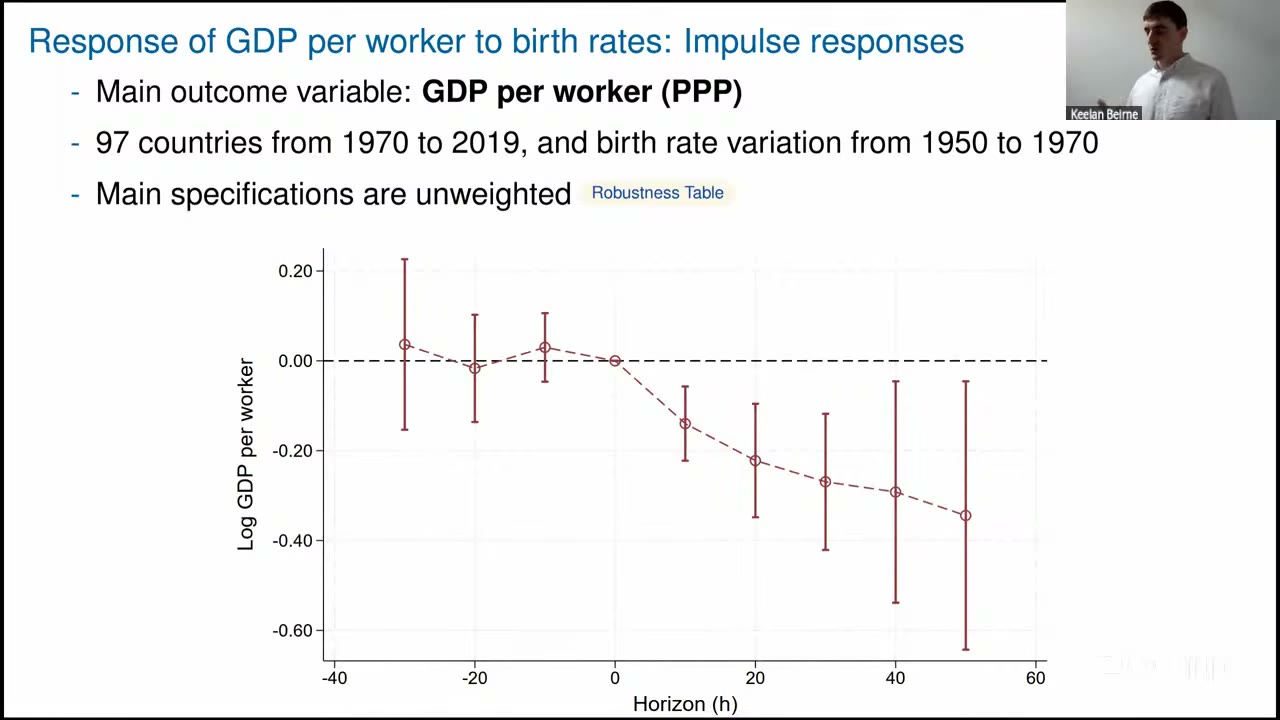
The impulse response is the talk’s main exhibit, and it works as its own placebo. For the twenty years before the cohort reaches working age there is nothing, and then, as Beirne put it, “as soon as these people are old enough to enter into the labor force,” gdp per worker starts to fall. The paper reads it as 22 log points at $t+20$ and 29 at $t+40$ for a one-point lower birth rate, about 0.73 percentage points of extra growth a year (p. 21). The talk rounded this to “30% higher gdp about 70 years after the birth rate happens” (01:43:48). For scale, one percentage point of crude birth rate is about half of the entire global decline since 1950, which Beirne called “very very large but also in the support of our data.” (The slide says 97 countries, 1970–2019. The paper’s Table 1 uses 107, and it never gives the sample size for the local projection. The slides probably predate the draft.)

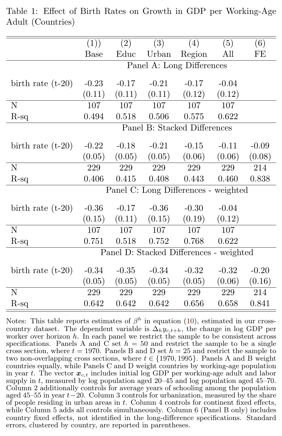
In the regression tables, the baseline long difference is −0.23 (0.11), N = 107, and the stacked 25-year version is −0.22 (0.05). Weighting by population makes the estimates larger, at −0.36 and −0.34. The honest reading of Table 1 is that the result survives controls for education, urbanization and region one at a time, but not all together (−0.04, s.e. 0.12), and that country fixed effects cut the stacked estimate to −0.09 (0.08), which is not significant. The paper does not hide these columns. It also reports the same 1950-to-1970–2020 regression three different ways. Figure 2A gives −0.268 (0.113), which is where the introduction’s “26.8% higher” comes from; it uses 1970–2019 growth rescaled to 50 years. Table 1 gives −0.23 with 2020 imputed. Appendix Table A1 gives −0.13 (0.10) with N = 120. The samples and endpoints differ and the paper never reconciles them. The text uses −0.23, and so does this note.

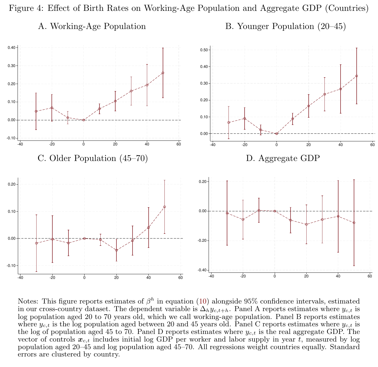
Figure 4 is the result that matters most, and the rest of the paper follows from it. Working-age population falls about 16 log points by $t+30$ for a one-point lower birth rate (and about 25 after 70 years), yet aggregate gdp (panel D) shows nothing. In the appendix, Table A4 has the long difference at +0.02 (0.14). The paper then does the arithmetic. With $s_L \approx 0.6$, the direct loss is $0.6 \times 0.16 \approx 9.6$ log points, and technology and capital have to make that up (p. 23). “Whatever those technology responses are,” Beirne said, “they’re sufficient to keep aggregate income constant” (01:45:35).

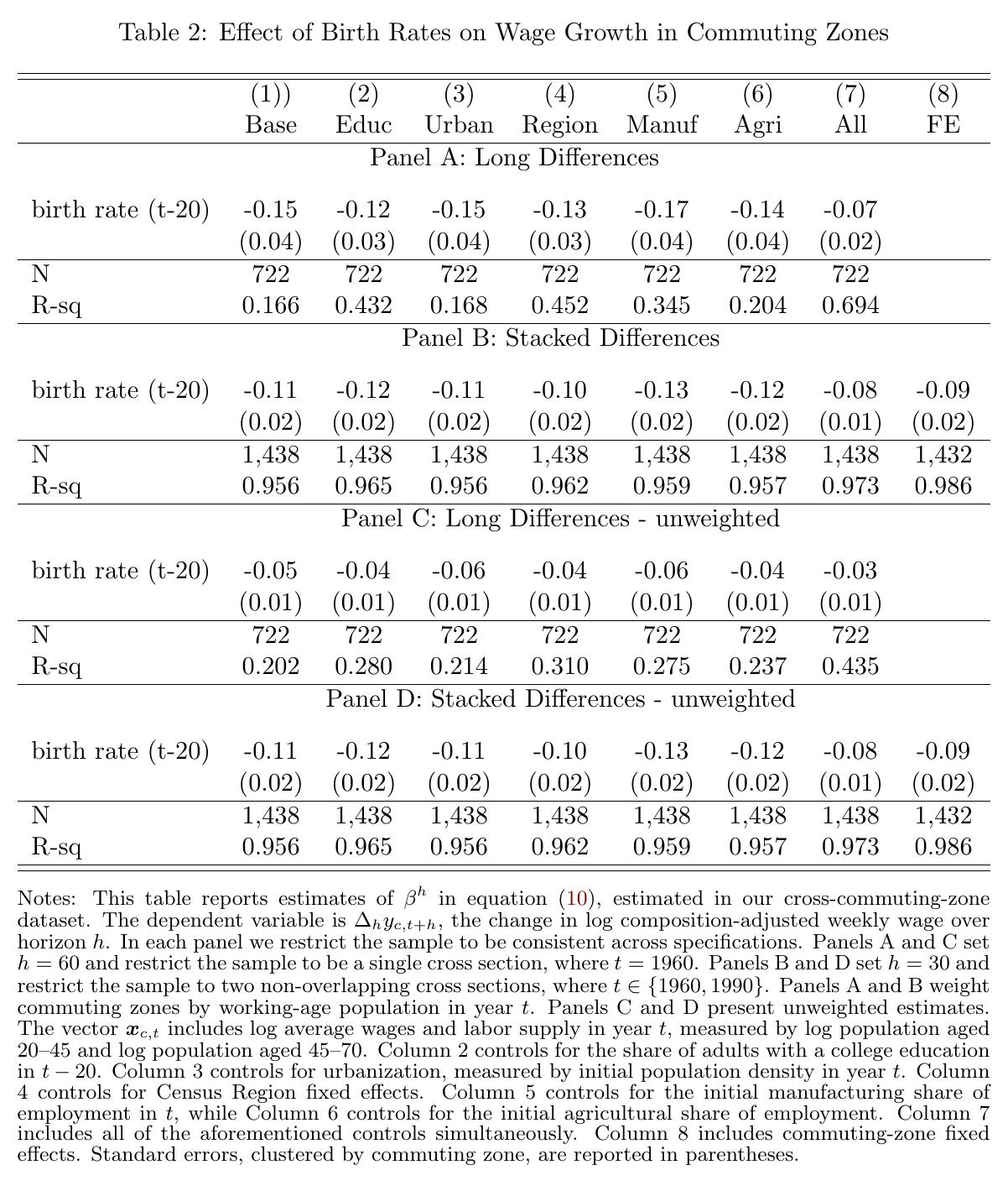
The commuting zones give the same sign at about half the size. Across 722 zones, weighted, a one-point lower 1940 birth rate means 15 log points more composition-adjusted wage growth from 1960 to 2020, −0.15 (0.04). The stacked version is −0.11 (0.02), with all controls it is −0.07 (0.02), and with zone fixed effects it is −0.09 (0.02) (Table 2, p. 24). The nice thing is that the accounting predicts the gap. Birth rates are much less persistent across zones than across countries (Fig. 7), so zone employment falls only about 7 percent instead of 16. The hole is therefore about $0.07 \times 0.6 \approx 4.2$ percent, not 9.6, and the induced response is correspondingly smaller (p. 27). The talk’s slide said 716 zones and 2019, and it described the zone birth-rate window as “1914 and 1970,” which is presumably the captions garbling 1940. (In the table, Panel D is labelled unweighted but reprints Panel B digit for digit; the unweighted long difference in Panel C is a smaller −0.05.)

Where the robots show up

If technology filled the hole, you should be able to see it. Country tfp is 15 log points higher by $t+30$ after a one-point lower birth rate (Fig. 10A, p. 31), which is more than the 9.6 that is needed. (Appendix Table A7 puts it at about 24. The sign is the same, the magnitude is not reconciled.) Taken at face value, that overfills the hole. tfp plus a positive capital response ought to show up as aggregate gdp rising, and Figure 4D doesn’t show that. The paper counts the extra as sufficiency, not as an accounting loop that fails to close. Patenting moves the way the model says it should. After a higher birth rate, the ict share of patents falls by about 0.10 in countries and 0.14 in commuting zones, the automation share falls by an imprecise 0.07, and the patent share of labor-intensive industries falls even though those industries’ employment is growing (Table A8). Beirne called this last one “very indicative” of labor-saving technical change. Across commuting zones, a higher birth rate raises the employment share of labor-intensive industries and cuts the R&D-intensive share, and the latter shrinks “quite a lot” given how small it is (Fig. 9; 01:49:30). Table A7 prints those two coefficients with the signs reversed, which looks like swapped column headers; the figure and the text agree with each other.

The alternatives are dealt with briskly (Section 8): female participation moves the wrong way, schooling is too small (2 points of college share times a 75 log-point premium is about 1.5 log points, against more than 10; p. 35), and structural change has inconsistent signs.

The war

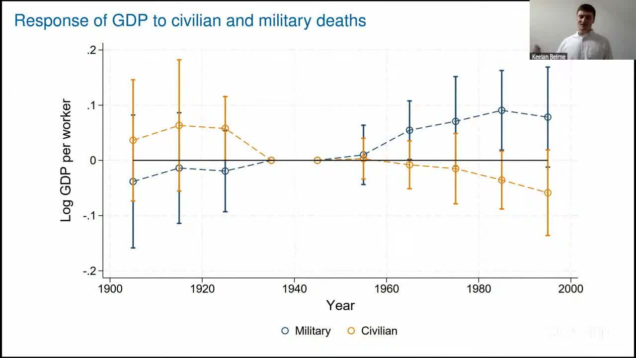
To separate aging from shrinking, the paper turns to what Beirne called “somewhat morbid variation” (01:52:09). Military deaths in the Second World War removed young men. Civilian deaths were spread roughly evenly across ages. The first shock ages a population and the second only shrinks it.

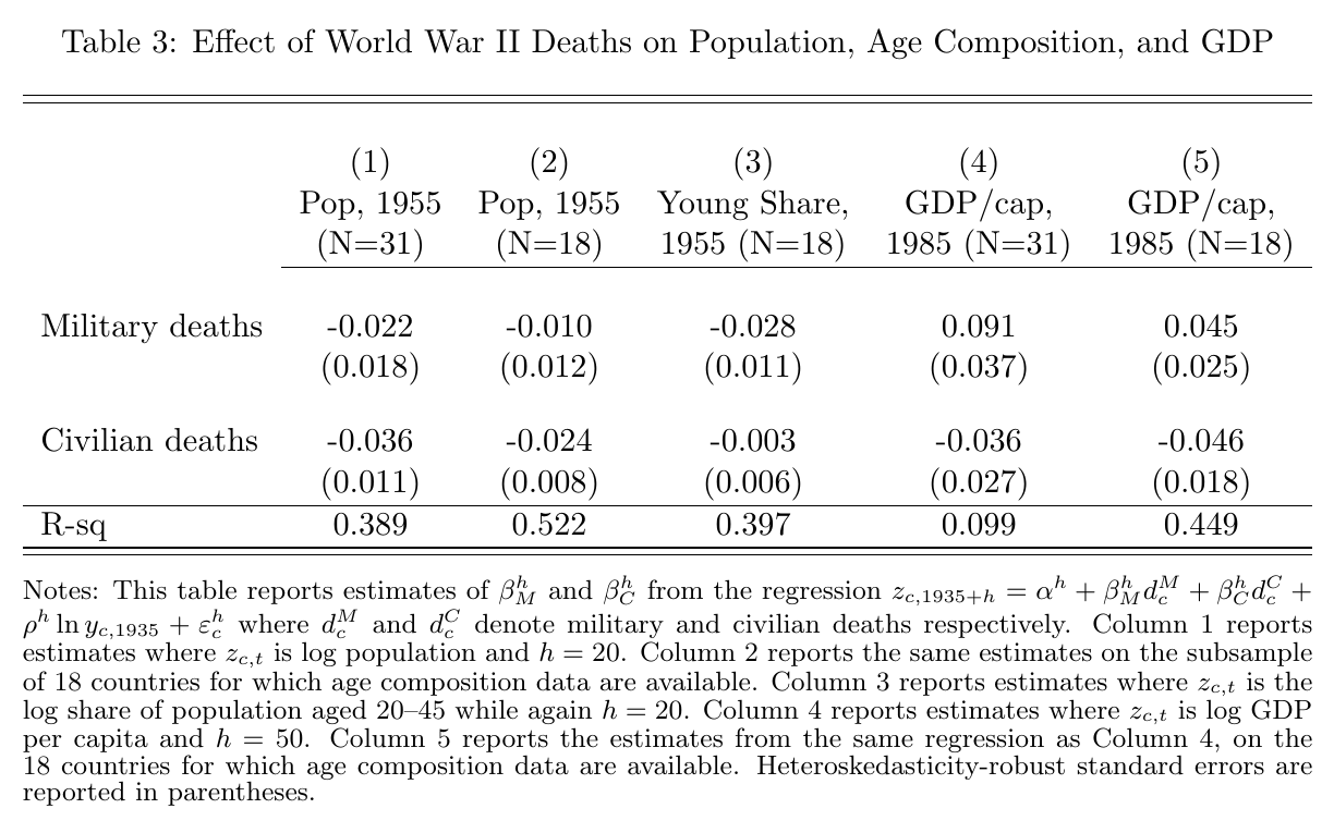
The first stage behaves. A point of military deaths lowers the 1955 young share by 2.8 log points (0.011), and a point of civilian deaths lowers it by only 0.3 (0.006). Then comes the result: forty years on, in 1985, military deaths predict gdp per capita 9.1 log points higher (0.037) and civilian deaths predict it 3.6 lower (0.027), with no pre-trend over 1905–35 (Table 3, p. 39). So losing young men made countries richer per head, and losing people in general made them poorer. The samples are 31 countries, or 18 with age data. In the full sample the civilian coefficient is not significant, and in the 18-country sample the military coefficient halves to 0.045 (0.025). The paper’s own word for all this, “suggestive,” is the right one. The talk version differs in several details. It said 22 countries, 1910–1995, “10% higher gdp by 1995,” with an axis labelled gdp per worker. The paper uses gdp per capita because working-age counts aren’t available (p. 38), and its introduction promises a “total war deaths” result that Section 9 never reports.

The room

A questioner the chair called Diego asked two things. First, birth rates drive both the demographic dividend and aging, so how can those be separated? Beirne answered that birth rates explain most of the change in population structure, that the reduced form bundles everything, and that the war is a first step with limited power. Second, would poorer countries that are aging fast also gain? Preliminary heterogeneity work, not in the paper, finds effects that are “if anything” larger in lower-income countries, which have more room for labor-saving change (01:58:48). A second questioner, not introduced, brought up urban economics: density raises productivity and cities have low fertility, so is this agglomeration running backwards? Beirne’s reply was that density and urbanization controls change nothing, that us birth rates are not a map of rural versus coastal, and that commuting-zone ols of wages on population comes out at about zero because migration arbitrages wages away. That last point is the reason to use births in the first place (02:02:03).

James raised Peters and Walsh (2026), where population decline gives short-run gains and the semi-endogenous scale effect wins in the long run. Is this just the transition? Beirne answered that the estimates are still growing at 70–80 years with no sign of turning back. A lower birth rate means a permanently older stationary population, so young wages stay permanently higher and technology stays permanently more advanced, and the war evidence says the scale effect is real but dominated (02:04:07). Fair, though 70 years is not long by the standards of a semi-endogenous transition. A questioner the chair called Adrian (presumably Adrien Auclert, one of the organisers) raised the missing intercept. If labor-saving innovations diffuse, the cross-section cannot see the global response. Beirne conceded the point, and Adrian then noticed that the concession cuts in the paper’s favour: the global effect would be larger than 30 percent. “I think that’s exactly right,” Beirne said (02:08:03). It is not every day that a missing-intercept objection ends with the author agreeing the result is bigger.

Last came a questioner the chair called Larry. The us saved 1.5 percent of national income last year and invested 6.5 percent net, so foreigners own a growing share of the capital, and gdp per capita could rise while Americans’ national income falls; the us would be “looking more like Jamaica where all the hotels are owned by foreigners” (02:08:42). Beirne agreed that the object is production, not welfare or gni, though “if your productivity goes up by 30%, you probably do gain.” Then he added the sentence the whole paper could carry as its disclaimer: “a us sovereign default never happened in the support of our data” (02:10:49).

Which is the right place to end up. The historical record says that when young workers got scarce, someone built the machine to replace them, and the machine was worth about as much as the missing workers. The coming transitions, in China especially, are faster than anything in the sample, and the paper says so. What the evidence does support is the robots. Who owns them is Larry’s question, and the paper leaves it open.

References