Long-Run Effects of H-1B Immigration on the U.S. Economy

Ran Abramitzky, Leah Platt Boustan, Ahmet Gulek and Jens Hainmueller

Presented by Ahmet Gulek at the nber Economics of Talent Conference, Cambridge ma, 2 October 2026 (video). No discussant.

Paper version: the July 2026 nber working paper (No. 35560). The deck Gulek presented looks newer than that paper in several places, and the note says which source each number comes from.

The political fight over H-1B visas is a fight about programmers. An Indian software engineer arrives, an American software engineer either loses a job or takes a lower wage, and you argue about whether that trade is worth it. This paper’s answer is that the American programmers come out roughly flat. The people who gain are their non-Stem coworkers, the immigrants who were already here, and, a bit more faintly, the people who work in insurance. The authors’ summary, on Gulek’s last slide (02:23:04): “H-1B is not only immigration policy. It is technology policy.” That is a recategorization, and the paper’s job is to show that it is true and not just a slogan. Its argument is that the visa inflow behaved like a productivity shock to the industries that absorbed it, not just like extra labor.

Why industries

There are two standard ways to study H-1Bs, and the paper argues that each designs away the effect it cares about. Firm-level lottery designs compare firms that won the visa lottery with firms that lost it, so any spillover to other firms in the same industry is differenced out. (In the talk, Gulek frames this literature as a seesaw: Doran and co-authors find native displacement, Mahajan and co-authors find none. The paper’s reading of Mahajan et al. is gentler. It says most incumbents gain there, and only high-tenure native college workers lose.) Cross-city designs compare places with many H-1Bs to places with few, which differences out the national general-equilibrium response. The paper estimates this “missing intercept” at roughly 40 percent of the total effect (p. 4).

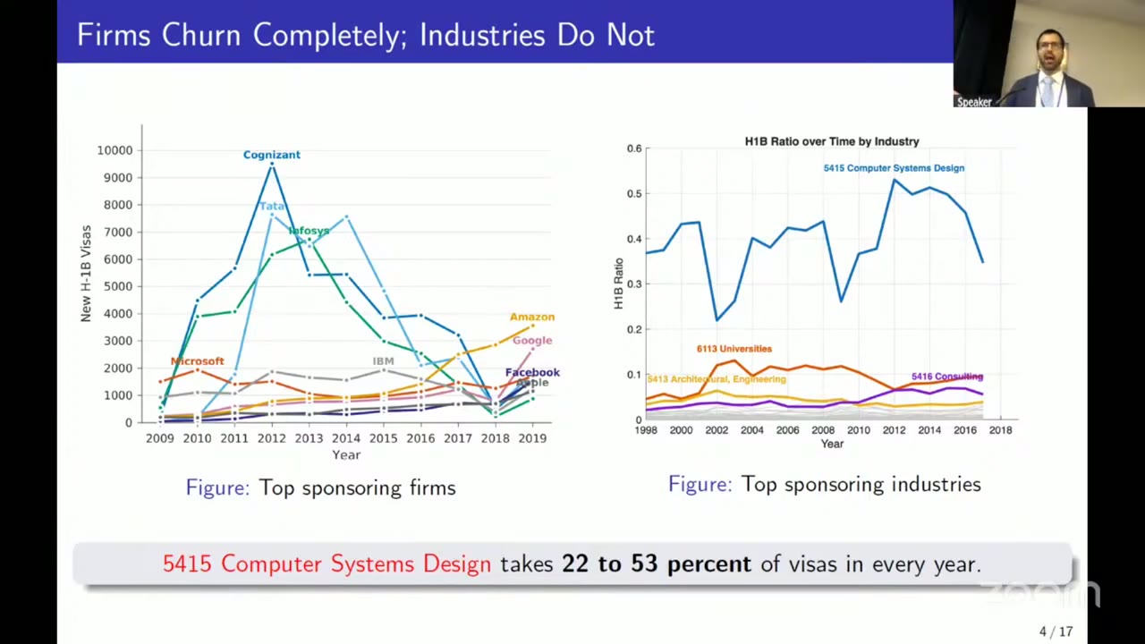
So the authors go up to the industry, for two reasons. First, the industries are where the persistent variation is. The firms change completely over time, but the industry ranking hardly moves at all:

Second, the United States publishes input-output tables only at the industry level, so if you want to follow a shock down the supply chain, the industry is the only unit you can use.

The shock is the cap. It went from 65,000 to 115,000 and then to 195,000 between FY1999 and FY2003, then fell back to 65,000 in FY2004 (plus 20,000 for U.S. master’s graduates from FY2005). That adds up to about 490,000 extra statutory visas. Each industry’s exposure is its 1998–2000 share of H-1B filings times that shift, measured as extra H-1B workers per 100 workers in 2000. This is a shift-share with exactly one shift, so identification has to come from the shares being exogenous. The 195,000 cap was never filled, so the estimates are intent-to-treat and, per realized worker, conservative.

The pre-trend problem, and what is done about it

The shares are obviously not random. The industries that hired H-1Bs in 1998 were the ones riding the dot-com boom, and plain difference-in-differences shows pre-trends you could see from across the room. The fix is what the paper calls sc-DiD, a synthetic control with a continuous treatment. For each industry, you build a synthetic twin from donors in the same college-share quartile, matched on the pre-2000 income path. You apply the same weights to the exposure variable, subtract the twin from the original on both sides, and run ols on what is left. (This is the reduced form of a synthetic-iv estimator by Gulek and Vives-i-Bastida; the talk credits it to the latter’s job-market paper.) The estimating equation, applied to the debiased data, is the paper’s eq. (4):

Here $y_{it}$ is log income of a worker group in industry $i$ in year $t$, $E_i$ is H-1B exposure, $f_i$ are industry fixed effects, $f_{q(i),t}$ are skill-quartile-by-year fixed effects, and $\beta_{SR}$ and $\beta_{LR}$ are the short-run and long-run effects relative to 2000.

The authors are honest about how much this buys. In a backtest on qcew data, run in years where nothing was treated so that any estimated “effect” is pure bias, sc-DiD removes 12 percent of the ols bias with two pre-periods and 53–57 percent with six or more. The paper’s own phrase is that the debiasing is “real but partial” (OA12). The acs, where the headline results live, has only three decennial pre-periods and is not backtested at all.

Inference is where the talk and the paper part ways. Gulek said that with only a few effective clusters, clustered standard errors “don’t work,” so the team uses randomization inference, following (probably) Ferman and Pinto (02:13:44). The July paper reports industry-clustered standard errors throughout. It uses a wild-cluster bootstrap for only one table, and it concedes in that table’s notes that clustered errors “overstate precision.” The confidence intervals on the slides are visibly wider than the paper’s.

Who gains

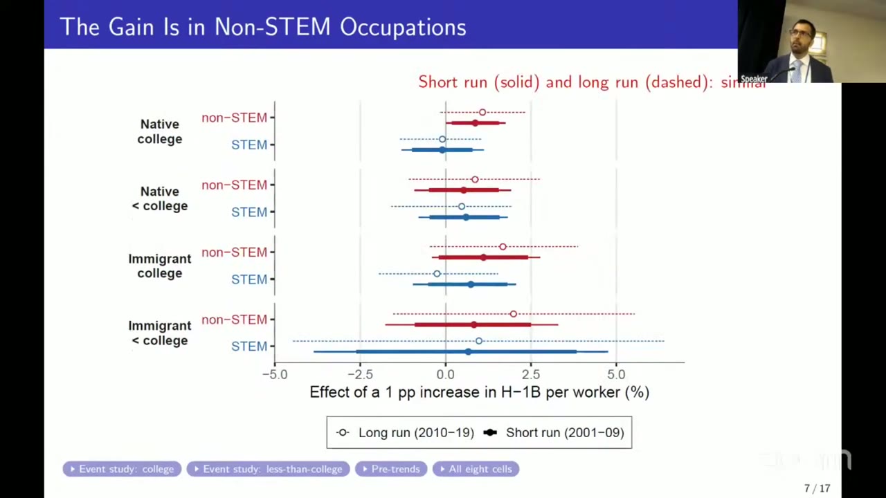
The headline number comes from the paper. One extra H-1B per 100 workers raises long-run income of native college graduates in non-Stem jobs by 1.16 log points (se 0.34). For native college graduates in Stem jobs, the estimate is −0.12 (0.07). In Computer Systems Design, the most exposed industry, the paper says this works out to roughly a 15 percent long-run gain for native non-Stem staff (p. 2). Pre-existing immigrants gain more than natives in most specifications, which is awkward for the story where new immigrants displace old immigrants and only complement natives. Gulek did not oversell the Stem estimate. He said it is “negative but super super small” and “not a precise null,” and that “we cannot rule out say minus 1%.”

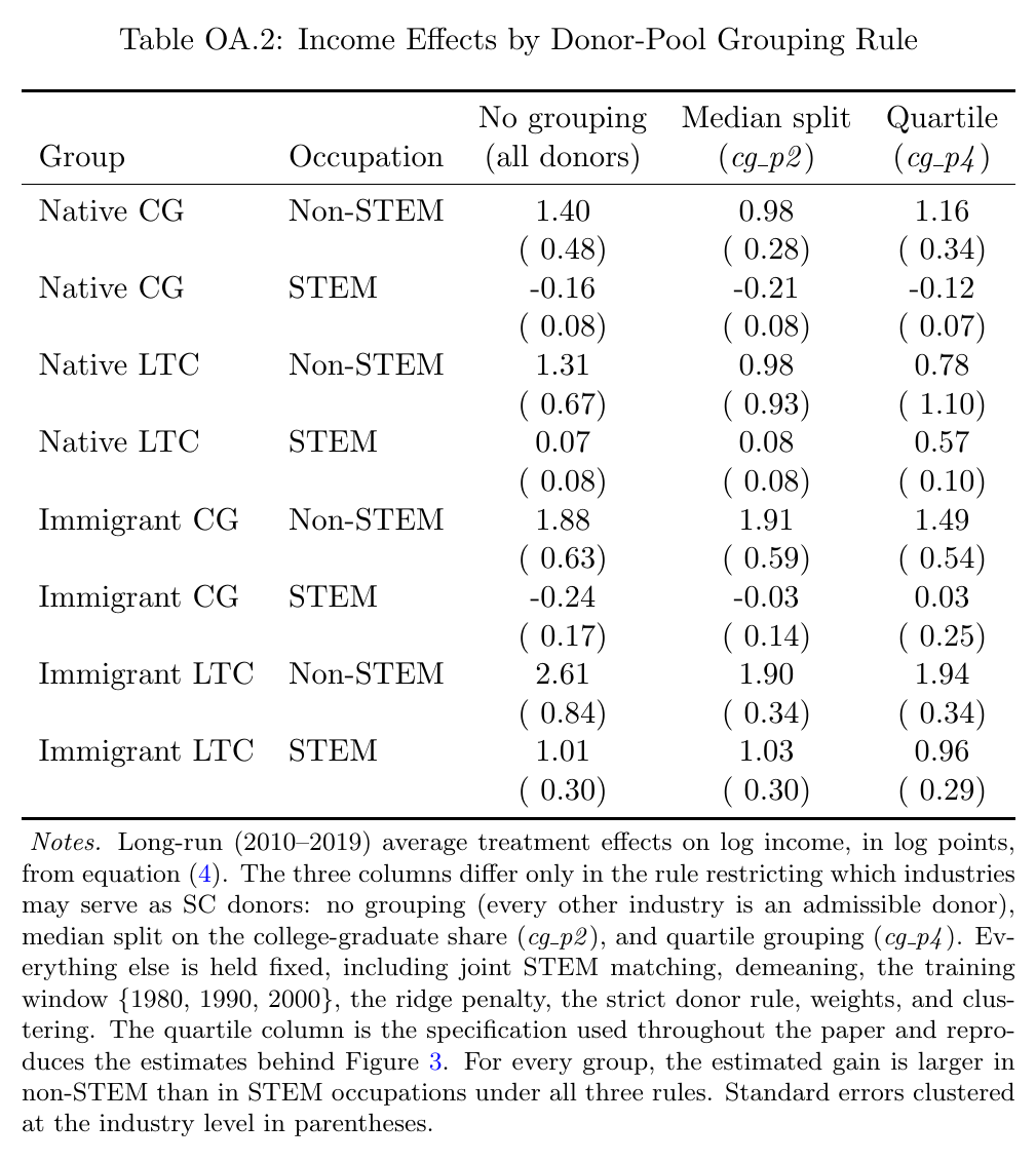
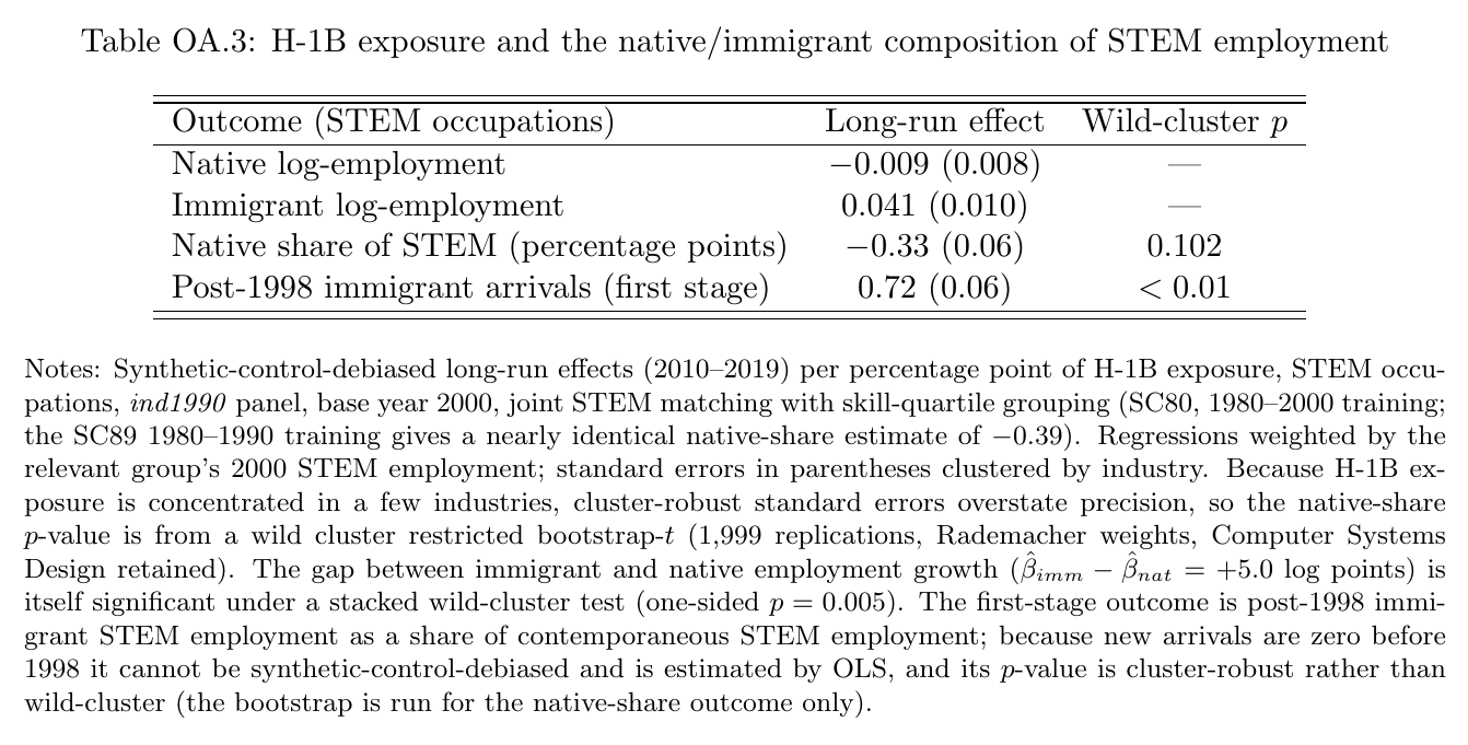
The Stem/non-Stem split also works as an identification test, which is the cleverest move in the paper. Suppose an unobserved technology boom drove both H-1B demand and incomes. Then the boom raises demand for Stem labor, and Stem wages should rise. What actually rises is the pay of the non-Stem coworkers, which is what you would expect if more Stem labor raises the marginal product of the people doing the complementary tasks. The composition data tell the same story. Native Stem employment is flat, immigrant Stem employment rises, and the native share of Stem jobs falls by 0.33 percentage points per point of exposure. The clustered standard error on that is 0.06, but the wild-cluster bootstrap p-value is 0.102, so the share result is suggestive rather than significant.

The forward/backward test

This is the paper’s distinctive argument, and it is where Gulek’s job-market paper (Gulek 2025) comes in. Take a chain of three industries: a supplier S sells to the exposed industry J, and J sells to a customer C. If J’s output gets cheaper, C benefits, whether J got cheaper because labor got cheaper or because J got better at its work. So forward propagation cannot tell the two stories apart. Backward propagation can. Under Cobb-Douglas final demand, expenditure shares are fixed, so a more productive J does not gain market share and does not buy more from S. A labor-supply shock, by contrast, changes J’s mix of labor and intermediate inputs, so it moves J’s purchases from S. Forward-only propagation therefore points to productivity. The exposures are built from the 1997 bea Leontief inverse, with the diagonal zeroed (eqs. 5–6):

Here $\Psi_{ij}$ is the Leontief-inverse entry with $i$ as buyer and $j$ as seller, so $F_i$ measures how H-1B-exposed $i$’s suppliers are and $B_i$ how exposed its customers are. The most directly exposed industry (Computer & Data Processing) is dropped from this sample.

In the paper, forward exposure raises long-run income by 10.9 log points for all workers (p = 0.039) and 9.7 for natives (p = 0.053). The short-run numbers are 6.8 and 7.6. Backward exposure is indistinguishable from zero. To scale that: compare a worker in insurance (forward exposure 0.38) with one in child day care (0.23). The insurance worker gained 1.0 percent more over 2001–09 and 1.6 percent more over 2010–19 (p. 13). That is not huge, but it reaches everyone who buys software, which is everyone.

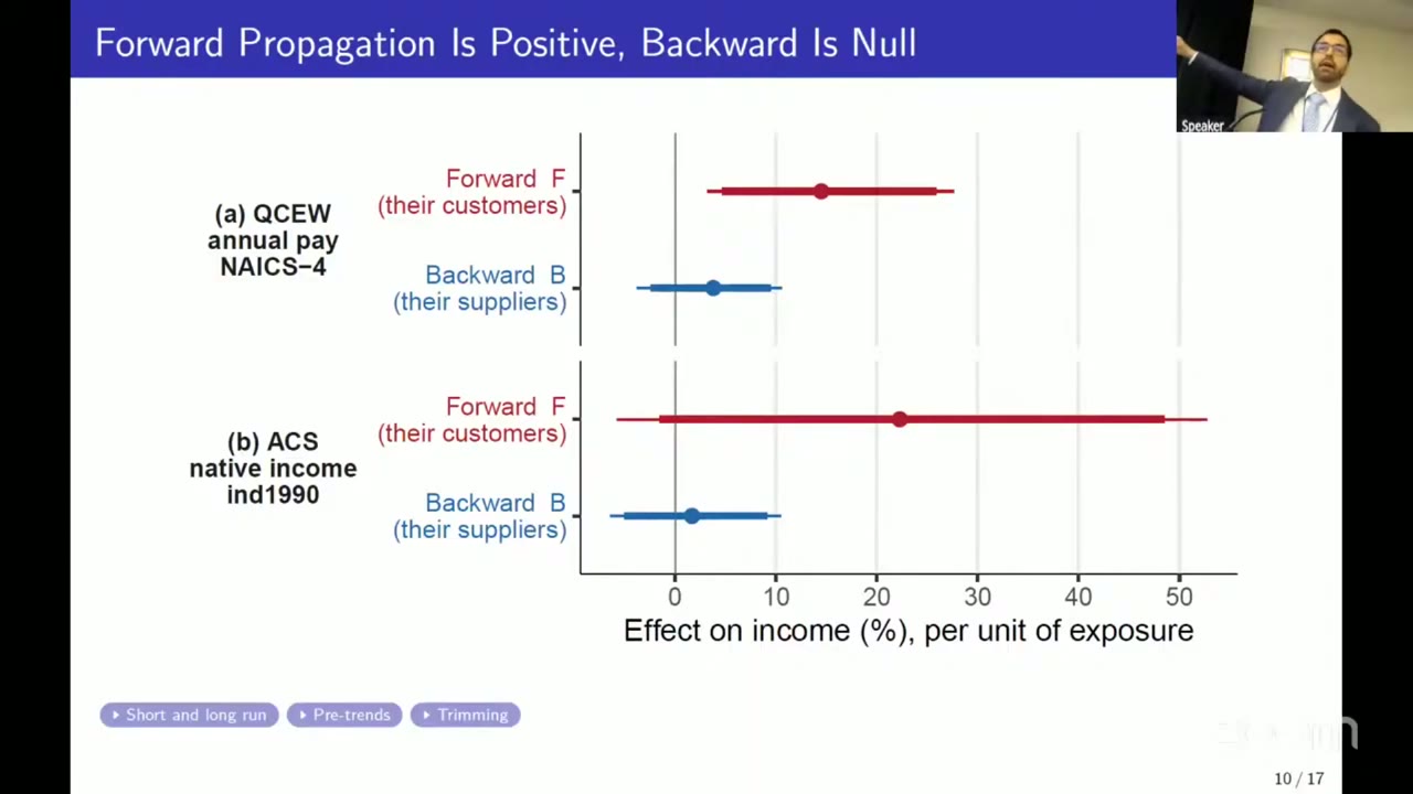
The slide’s numbers are not the paper’s. The acs forward estimate on the slide is around 22, and its interval crosses zero. The qcew panel’s point estimates, which are the ones that clear zero, do not appear in the July paper, which shows the qcew only as an event study. Gulek was careful to say the forward effect is significant “in the qcw.”

Then the talk does something the paper does not. It uses a model where labor and intermediates are gross complements, in which each pure shock has a signed backward prediction. Under a pure labor-supply shock, J’s labor gets cheaper and, because inputs complement labor, J buys more from S, so the backward-to-forward ratio $\beta_B/\beta_F$ is 1.5 in the qcew calibration (slide 02:18:01). Under a pure productivity shock, C faces cheaper inputs, shifts its spending toward labor and cuts its whole input bill. J then sells less and buys less from S, so the ratio is −0.7 (slide 02:19:40). The qcew data say 0.26, which rejects both. So the inflow is a mixture. You invert the model curve to find how much productivity, $\chi$, comes attached to each percent of extra labor:

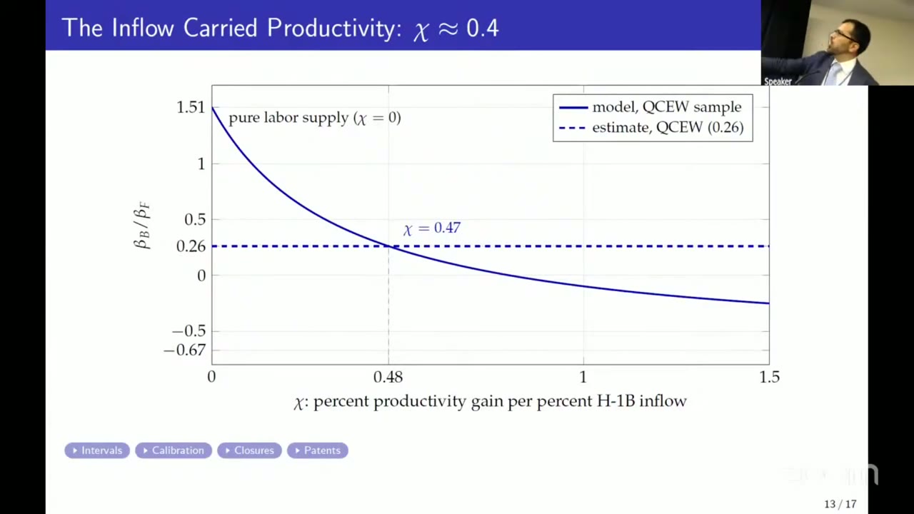
The qcew gives $\chi = 0.47$ and the acs about 0.33, and Gulek averaged them to “0.4.” Neither $\chi$ nor the 1.5 / −0.7 / 0.26 ratios appear in the July paper, and the functional form of the curve sits behind a “Calibration” backup button that was not shown.

It is worth being clear about what this curve depends on. In the paper’s own theory appendix (OA16–17), dropping Cobb-Douglas reopens a business-stealing route: a more productive J gains market share, scales up, and buys more from S. Under that route, a pure productivity shock propagates backward positively. The talk’s model gets a negative sign from a different elasticity, the labor-intermediate complementarity inside C. Both channels can exist at once. So the endpoint that pins $\chi$ is a statement about which elasticity wins, and the authors have not estimated those elasticities. The paper says so itself: it calls the test “suggestive rather than dispositive,” and notes that a zero backward estimate could be two spillovers cancelling. The talk tells the same cancelling story (02:20:05), but with signs chosen so that the cancellation measures something. That is a reasonable thing to try. It is also a structural number resting on a model the paper does not contain.

Not patents

If H-1Bs raised productivity, where did it come from? Not from patents. With sc-DiD, log patents and citations in exposed industries are flat to slightly negative after 2000. The authors also take apart the Kerr–Lincoln regional result instead of just disagreeing with it. By 2019, patenting in states with above-median H-1B intensity is 0.56 log points above the rest. Split by industry, Computer Systems Design ends only 0.29 apart (its patenting actually fell in the high-exposure states), and industries with essentially no H-1B workers end 0.74 apart. The regional patent boom is real, but it comes from industries that do not hire H-1Bs. Gulek’s version: a superstar software engineer in 2000 makes the software better and is “not going to patent it,” and everyone downstream runs on the better software.

The bill for ending it

The policy hook is the $100,000 fee on new petitions for workers entering from outside the U.S.. Gulek showed a September 2026 headline about H-1B demand plummeting after it. He then did a back-of-envelope that exists only in the talk (slide 02:22:07). Admitting 85,000 fewer H-1Bs a year cuts labor supply in computer services by 1.1 percent. That cuts productivity there by 0.5 percent, which is roughly $\chi$ times the labor number, as it should be. It also cuts native non-Stem college-graduate income there by 1.2 percent, and income in customer industries by 0.5 percent on the 1997 network or 0.7 percent on the 2017 network. The slide has a question mark for 2025, on the theory that ai makes computer services more central still. Gulek said these losses accumulate “more or less linearly” year after year. (A spoken real-gdp figure was garbled by the captions and is not on the slide, so it is left out.) The paper’s conclusion says only that restrictions “could dampen productivity gains,” with no numbers.

Q&A

An unnamed questioner put the obvious objection directly (02:23:48): isn’t this just an it-industry shock, so that without it the results would vanish? Gulek split his answer. The forward/backward estimates already exclude the computer industry, so they come only from industries that are not directly exposed. For the direct effects, “you are absolutely right.” Without that one industry the intervals become so wide that you cannot rule out a null, nor rule out that the effect differs from computer science’s. He said that is exactly why clustered errors fail and randomization inference is needed. The paper agrees, noting that dropping industry 732 “would remove most of the identifying variation by construction” (OA10). So the direct-effect results rest largely on one industry and its synthetic twin.

A second questioner asked whether the data can separate H-1Bs for people already in the U.S. from new arrivals, which matters because the $100,000 fee applies only to entries from abroad. The whole answer: “Great question. Absolutely not. I wish.”

Gulek closed by noting that he is on the job market and needs an H-1B himself. By the paper’s estimates, whoever hires him should expect most of the benefit to show up in their colleagues’ pay.